Báo cáo sinh học: "Genome-assisted prediction of a quantitative trait measured in parents and progeny: application to food conversion rate in chickens" potx
Bạn đang xem bản rút gọn của tài liệu. Xem và tải ngay bản đầy đủ của tài liệu tại đây (482.57 KB, 10 trang )
BioMed Central
Page 1 of 10
(page number not for citation purposes)
Genetics Selection Evolution
Open Access
Research
Genome-assisted prediction of a quantitative trait measured in
parents and progeny: application to food conversion rate in
chickens
Oscar González-Recio*
1
, Daniel Gianola
1,2
, Guilherme JM Rosa
1
,
Kent A Weigel
1
and Andreas Kranis
3
Address:
1
Department of Dairy Science, University of Wisconsin, Madison, WI 53706, USA,
2
Department of Animal Sciences, University of
Wisconsin, Madison, WI 53706, USA and
3
Aviagen Ltd., Newbridge, Scotland, UK
Email: Oscar González-Recio* - ; Daniel Gianola - ; Guilherme JM Rosa - ;
Kent A Weigel - ; Andreas Kranis -
* Corresponding author
Abstract
Accuracy of prediction of yet-to-be observed phenotypes for food conversion rate (FCR) in
broilers was studied in a genome-assisted selection context. Data consisted of FCR measured on
the progeny of 394 sires with SNP information. A Bayesian regression model (Bayes A) and a semi-
parametric approach (Reproducing kernel Hilbert Spaces regression, RKHS) using all available SNPs
(p = 3481) were compared with a standard linear model in which future performance was predicted
using pedigree indexes in the absence of genomic data. The RKHS regression was also tested on
several sets of pre-selected SNPs (p = 400) using alternative measures of the information gain
provided by the SNPs. All analyses were performed using 333 genotyped sires as training set, and
predictions were made on 61 birds as testing set, which were sons of sires in the training set.
Accuracy of prediction was measured as the Spearman correlation ( ) between observed and
predicted phenotype, with its confidence interval assessed through a bootstrap approach. A large
improvement of genome-assisted prediction (up to an almost 4-fold increase in accuracy) was
found relative to pedigree index. Bayes A and RKHS regression were equally accurate ( = 0.27)
when all 3481 SNPs were included in the model. However, RKHS with 400 pre-selected
informative SNPs was more accurate than Bayes A with all SNPs.
Introduction
Genome-wide association studies of diseases and com-
plex traits [1] have permeated into animal breeding, and
genome-assisted selection has become a major focus of
research [2,3]. However, genome-based artificial selection
poses several challenges. For instance, methods for predic-
tion of genetic merit or phenotype using a large number
of markers must be contrasted and improved. Also, bio-
logical and economical advantages of genome-assisted
selection in a breeding program must be quantified (this
second problem is not addressed herein).
Published: 5 January 2009
Genetics Selection Evolution 2009, 41:3 doi:10.1186/1297-9686-41-3
Received: 16 December 2008
Accepted: 5 January 2009
This article is available from: />© 2009 González-Recio et al; licensee BioMed Central Ltd.
This is an Open Access article distributed under the terms of the Creative Commons Attribution License ( />),
which permits unrestricted use, distribution, and reproduction in any medium, provided the original work is properly cited.
r
S
r
S
Genetics Selection Evolution 2009, 41:3 />Page 2 of 10
(page number not for citation purposes)
A very important issue is how to deal with a much larger
number of markers (p) than of individuals that are geno-
typed (n). Some proposals include treating marker effects
as random, with shrinkage of estimates of non-informa-
tive markers to zero. This is done naturally in a Bayesian
context, where all unknowns are treated as random varia-
bles (e.g., Gianola and Fernando, [4]). On the one hand,
Bayesian regression methods, such as Bayes A and Bayes B
[2], or the special case of Bayes A described by Xu [5] have
recently gained attention. However, all of these proce-
dures involve strong assumptions a priori. On the other
hand, non-parametric methods have been suggested as an
alternative for predicting genomic breeding values,
because these methods may require weaker assumptions
when modeling complex quantitative traits [6].
These non-parametric approaches have been applied to
simulated [7] and field [8] data, and results seem promis-
ing. The simulations from Gianola et al. [7] involved 100
biallelic markers and additive × additive interactions
between five pairs of loci. Gonzalez-Recio et al. [8] used
24 pre-selected SNPs from a filter and wrapper feature
subset selection algorithm [9] in a reproducing kernel
Hilbert spaces (RKHS) regression model. However, these
non-parametric methods have not been tested yet using a
large number of SNPs and field data. Inclusion of a large
number of SNPs in these non-parametric models must be
studied. Further, evaluating the accuracy of such methods
in predicting phenotypes in future generations is a crucial
issue in artificial selection programs.
Genomic information became available in animal breed-
ing recently, and most research involving either the large
p small n problem [10,2] or the prediction of future gen-
erations [11,12] has resorted to simulations. Arguably,
assumptions built in simulations may fail to represent the
true complexity of biological systems and, typically, sim-
ulations tend to favor some of the models under evalua-
tion. Therefore, the extent to which simulation results
hold with real data can be questioned.
The present paper uses field data from the Genomics Ini-
tiative Project at Aviagen Ltd. (Newbridge, UK). Food con-
version rate (FCR) is one of the most economically
important traits in the broiler industry, because it affects
feeding and housing costs markedly. Genome-assisted
selection programs may provide greater reliability of pre-
dictions of future performance, thus increasing profitabil-
ity.
The objective of this study was to compare the ability of
Bayes A regression and of semi-parametric (RKHS) regres-
sion to predict yet-to-be observed phenotypes, using field
data on FCR in a two-generation setting.
Methods
Animal Care and Use Committee approval was not
obtained for this study because the data were obtained
from an existing database supplied by Aviagen Ltd. (New-
bridge, UK).
In a nutshell, a one-fold cross-validation with a training
set and a testing set was carried out, as the testing set
included only sons of sires that were in the training test.
Several statistical methods were used to predict the aver-
age phenotypes of offspring of animals in the testing set,
i.e., first-generation performance. These included a stand-
ard genetic evaluation, which ignored SNP genotypes, and
two methods that included all available SNPs (after edit-
ing) as predictors in the model. The latter methods, which
included genomic information, were Bayesian regression
and RKHS regression. In addition, the RKHS regression
approach was fitted with 400 pre-selected SNPs, where
pre-selection was based on information gain using alter-
native criteria. In this section, the data set employed, the
pre-selection of SNPs, and the statistical methods that
were applied are described.
Phenotypic Data
Data consisted of average FCR records for progeny of each
of 394 sires from a commercial broiler line in the breeding
program of Aviagen Ltd. Prior to the analyses, the individ-
ual bird FCR records were adjusted for environmental and
mate effects, as described in Ye et al. [13]. In order to
assess the reliability of genome-assisted evaluation, two
data sets (training and testing) were constructed. The test-
ing set included offspring from sires with records in the
training set. Sires included in the testing set were required
to have sires in the training set with progeny records, and
needed to have more than 20 progenies with FCR records,
to have a reliable mean phenotype. Sires in the training
and testing sets had an average of 33 and 44 progeny,
respectively. Family size (half sibs) in the training set
ranged between 1 and 284, with the mean and median
being 32 and 17, respectively. Sixty-one sires (15.5% of
the total) were included in the testing set, whereas the
remaining 333 sires were in the training set. Predictions
were calculated from the training set, and the accuracy of
predicting the mean progeny phenotype was assessed
using sons in the testing set.
Genomic Data
Genotypes consisted of 4505 SNPs chosen from the 2.8
million SNPs identified in the sequencing project of the
chicken genome [14]. A data file titled "Database of SNPs
used in the Illumina Corp. chicken genotyping project"
(downloadable from />resources/resources.htm) describes partially the panel
used, and further details on the 6 K panel can be found in
Andreescu et al. [15]. All SNPs with monomorphic geno-
Genetics Selection Evolution 2009, 41:3 />Page 3 of 10
(page number not for citation purposes)
types or with minor allele frequencies less than 5% were
excluded. After editing, genotypes consisted of 3481 of the
initial 4505 SNPs.
Pre-selection of SNPs to be included in the analyses was
performed using the information gain or entropy reduc-
tion criterion [16,9]. Information gain is the difference in
entropy of a probability distribution before and after
observing genotypes, i.e., it measures how much uncer-
tainty is reduced by observation of SNP genotypes. The
entropy of the probability distribution of a discrete ran-
dom variable Y is defined as:
where A is the set of all states that Y can take, and the log-
arithm is on base 2 to mimic bits of information. The
above pertains to a discrete distribution since entropy is
not well defined in the continuous case [17]. Here, Y refers
to FCR phenotypes that were discretized by considering
different number of classes of FCR and different cutpoints,
as follows. First, two extreme FCR classes ("low" and
"high") were set up using cutpoints corresponding to the
and (1-) quantiles ( = 0.15, 0.20, 0.25, 0.35 and
0.40) of the FCR phenotypes for sires in the training set.
Further, an additional "middle" class (FCR between per-
centiles 0.40 and 0.60) was included to enrich the discre-
tized data. In total, information gain was calculated in ten
subsets, corresponding to combinations of the five
'extreme' tail -values, with or without the intermediate
class.
For each SNP, the training set was divided into three sub-
sets corresponding to the three possible genotypes (aa, Aa
or AA). For each genotype k there are sires with gen-
otype k in the high class, sires with genotype k in the
low class, and possibly sires with genotype k in the
middle class, if included. The information gain for each
SNP s (s = 1,2, , 3481) was the change in entropy after
observing the genotypes, calculated as:
where . Note that = 0 if a mid-
dle class was not included.
The 400 SNPs with largest information gain in each of the
ten partitions were pre-selected to build up a 400-SNP
genotype for each sire. Note that the choice of the 400
SNPs was arbitrary, but it roughly represents 10% of the
initial SNPs.
Models
Let y (333 × 1) be the vector of mean adjusted FCR records
for progeny of sires in the training set. Three different
methods for prediction of genomic breeding values for
FCR were used, as described next.
Standard genetic evaluation (E-BLUP)
A Bayesian equivalent of empirical best linear unbiased
prediction of sires' transmitting abilities, as described by
Henderson [18], was used. This method uses pedigree
data as the only source of genetic information. The linear
model was:
y =
1 + Zu + e
where,
is an unknown mean; 1 is a vector of ones; u =
{u
i
} is a vector of sire effects; u
i
is the effect of sire i in the
pedigree (i = 1, 2, , 624) and Z is an incidence matrix of
order 333 × 624 linking u to the observed data. A priori,
the sire effects were assumed to be distributed as u ~N(0,
A ), where A is the additive relationship matrix
between sires, and is the variance between sires. The
residuals, e, were assumed to be distributed as N(0, R = N
-
1
), where N = {n
i
} is a diagonal matrix with elements
n
i
representing the number of progeny of sire i and is
the residual variance. This dispersion structure for e
weights the residuals according to the number of progeny
each sire has [17,19]. Independent scaled inverted chi-
square prior distributions were assigned to the sire and
residual variances as and ,
respectively, where
u
= 5 and
e
= 3 correspond to the
degrees of freedom, and = 0.1 and = 8.67 were the
corresponding scale parameters. Sire merit (transmitting
ability) was inferred using a Gibbs sampling algorithm.
Bayes A
Meuwissen et al. [2] have proposed a Bayesian model in
which the additive effects of chromosome segments
marked by SNPs follow a normal distribution with a seg-
ment-specific variance. These variances are assigned a
common scaled inverted chi-square prior distribution.
The model fitted in this study had the form:
y =
1 + Xb + e.
HY y y
yA
(Pr( )) Pr( )log Pr( ),=−
∈
∑
2
N
k
H
N
k
L
N
k
M
IG SNP H
N
k
C
CLMH
N
N
k
C
N
N
k
C
N
i
CLMH
( ) (Pr( ))
,,
log
,,
=−
=
∑
−
⎛
⎝
⎜
⎜
⎜
⎞
⎠
=
∑
Y
2
⎟⎟
⎟
⎟
⎛
⎝
⎜
⎜
⎜
⎜
⎞
⎠
⎟
⎟
⎟
⎟
=
∑
k 1
3
,
N =+ +NN N
k
L
k
M
k
H
N
k
M
u
2
u
2
e
2
e
2
uuu
s
u
221
~
−
eee
s
e
221
~
−
s
u
2
s
e
2
Genetics Selection Evolution 2009, 41:3 />Page 4 of 10
(page number not for citation purposes)
Here, y is a 333 × 1 vector of progeny means for adjusted
FCR,
is their mean value, and 1 is a column vector of
ones; b = {b
s
} is a vector of 3481 × 1 SNP effects, and b
s
is
the regression coefficient on the additive effect of SNP s (s
= 1, 2, , 3481). Elements of the incidence matrix X, of
order n × p (n = 333; p = 3481), were set up as for an addi-
tive model, with values -1, 0 or 1 for aa, Aa and AA, respec-
tively. The b
s
effects were assumed normally and
independently distributed a priori as N(0, ), where
is an unknown variance specific to marker s. The prior dis-
tribution of each was assumed to be
-2
(
, S) with
=
4 and S = 0.01. The residuals (e) were assumed to be dis-
tributed as N(0, R), with R constructed as in the previous
model.
Reproducing kernel Hilbert spaces regressions
A RKHS regression [20-22] is a semi-parametric approach
that allows inference regarding functions, e.g., genomic
breeding values, without making strong prior assump-
tions. As described in Gianola and van Kaam [6] and
González-Recio et al. [8] in the context of genome-assisted
selection, this model can be formulated as:
y = X + K
h
+ e,
where the first term (X) is a parametric term with as a
vector of systematic effects or nuisance parameters (only
was fitted in this case, since the data were pre-corrected),
and X is an incidence matrix (here a vector of ones, 1). The
non-parametric term is given by K
h
, where K
h
is a posi-
tive definite matrix of kernels, possibly dependent on a
bandwidth parameter (h), and is vector of non-paramet-
ric coefficients that are assumed to be distributed as
, with representing the reciprocal of
a smoothing parameter ( =
-1
). The residuals e were
assumed to be distributed as e ~N(0, R), with R as for the
previous models. It can be shown that, given h and
, the
RKHS regression solutions satisfy the linear system:
There are two key issues in the RKHS regression pertaining
to the non-parametric term: choosing the matrix of ker-
nels, and tuning the h and
parameters. The matrix of ker-
nels aims to measure "distances" between genotypes. This
matrix K
h
had dimension 333 × 333, with rows in the
form , j = 1, 2, , 333, where K
h
(x
i
- x
j
)
is the kernel involving the genotypes of sires i and j. The
kernel refers to any smooth function for distances
between objects, such that K
h
(x
i
- x
j
) 0. Different types of
kernels may be used [23]. A Gaussian kernel was chosen
in this research, with form:
, where dist(x
i
- x
j
) is a
measurement of distance between genotypes of sires i and
j, and h is a bandwidth parameter. The choice of h and of
the measurement of distance between genotypes must be
done cautiously. A generalized (direct) cross validation
procedure was used to tune h, as described in Wahba et al.
[24]. However, measuring distances between genotypes is
less straightforward, because a large variety of criteria
might be used for this purpose (e.g. Gianola et al. [7];
Gianola and van Kaam, [6]; Gonzalez-Recio et al., [8]).
The algorithm used to measure distances between geno-
types is given next. Let x
i
and x
j
be string sequences of SNP
genotypes for sires i and j, respectively. These strings can
be separated into m substrings in which all SNPs differ
between the two sequences. For example, suppose x
i
=
(AABbCCDDEeFFGg), and x
j
= (AabbCcDDEeffgg). Here,
there are two substrings that differ from each other com-
pletely, corresponding to SNPs from loci 1–3, and 6–7
(table 1).
Then, compute the sum of the logarithms in base 2 (inter-
preted as bits of information) of the dissimilarity between
substrings. Dissimilarity was defined as the number of
alleles differing at each SNP. Hence, distance between two
genotypes can be expressed as:
where DA
k
is the number of different alleles in substring k.
In the example, sires i and j differ in one allele at each SNP
(AA vs Aa, Bb vs bb, and CC vs Cc) in substring 1. In sub-
string 2, sires i and j differ in 2 alleles for the first SNP (FF
vs ff) and in 1 allele for the second SNP (Gg vs gg). Here,
the two substrings had distances DA
1
= DA
2
= 3.
s
2
s
2
s
2
~(, )N
h
0K
−12
2
2
′′
′′
+
−
⎡
⎣
⎢
⎢
⎢
⎤
⎦
⎥
⎥
⎥
⎡
⎣
⎢
⎤
⎦
⎥
′
−−
−−
1R 1 1R K
KR 1 KR K K
11
11
1
1
h
hhh h
ˆ
ˆ
11R y
KR y
1
1
−
−
′
⎡
⎣
⎢
⎢
⎤
⎦
⎥
⎥
h
.
Table 1: Two substrings that differ from each other completely,
corresponding to SNPs from loci 1–3, and 6–7
Substring 1 Substring 2
Sire i AABbCC FFGg
Sire j AabbCc ffgg
′
=−
{}
kxx
ihij
K ()
K
hi j
dist
ij
h
( ) exp
()
xx
xx
−= −
⎛
⎝
⎜
⎞
⎠
⎟
−
dist DA
ij k
k
m
()log ,xx−= +
()
=
∑
2
1
1
Genetics Selection Evolution 2009, 41:3 />Page 5 of 10
(page number not for citation purposes)
A modification of this system was used for models in
which SNPs were pre-selected using the information gain
score. Here, the number of different alleles at each SNP
was weighted by the information gain score at that locus.
Therefore, the distance between two genotypes was calcu-
lated as: , where w
k
and da
k
are column vectors with typical elements equal to
the information gain score and the number of different
alleles, respectively, for each SNP in substring k. This ker-
nel weights dissimilarity between SNPs by the reduction
in entropy. With this approach, the kernel matrix K is
symmetric and positive definite, so it fulfills the require-
ments of a RKHS, and it can be viewed as a correlation
matrix between genomic combinations.
In total, 11 RKHS regression analyses were performed:
one including all 3481 SNPs; five ( = 0.15, 0.20, 0.25,
0.35 and 0.40) including 400 pre-selected SNPs using the
information gain calculated using two ("low" and "high")
classes to classify sires, and five ( = 0.15, 0.20, 0.25, 0.35
and 0.40) including 400 pre-selected SNPs with informa-
tion gain calculated by classifying sires into three ("low",
"medium" and "high") classes.
Posterior estimates from all models were obtained with a
Gibbs sampling algorithm based on 150,000 iterations,
discarding the first 50,000 as burn-in, and keeping all
100,000 subsequent samples for inferences.
Predictive ability
Progeny phenotypes in the testing set were predicted
using the estimates obtained from the training set. First,
using the training set with each model, inferences were
made regarding the predicted transmitting ability for E-
BLUP, prediction of SNPs coefficients for Bayes A, and
prediction of non-parametric coefficients for RKHS regres-
sion. Phenotypes in the testing set were predicted as fol-
lows:
E-BLUP
Phenotypes were predicted using pedigree indexes via sire
and maternal grandsire (information from maternal rela-
tives was not included). The pedigree index for sire t in the
testing set (PI
t
) was , where
PTA
s
and PTA
mgs
are the predicted transmitting abilities of
the bird's sire and maternal grandsire, respectively.
Bayes A
The p = 3481 estimates of regressions coefficients corre-
sponding to additive effects of the SNPs ( ) from the
training set were multiplied by their respective genotype
codes (x
ts
= -1, 0 or 1 for aa, Aa or AA, respectively) for sire
t in the testing set to obtain a predicted phenotype as
, where and are the posterior
means of
and b
s
, respectively.
Reproducing kernel Hilbert spaces regressions
Predictions were made using a matrix of kernels between
focal points (i.e., genotypes of sires in the testing set) and
support vectors (genotypes of sires in the training set) as:
where K* (h) is a matrix with dimension 61 × 333, and
with rows of the form , j = 1, 2, ,
333, where is the kernel between the geno-
type of sire t in the testing set and sire j in the training set.
The same bandwidth parameter that was tuned with the
training set was used. The vector represented the poste-
rior means of the 333 non-parametric regression coeffi-
cients for sires in the training sample.
Typically, the objective of prediction in animal breeding is
to rank candidates for selection, and to subsequently
choose the highest-ranked candidates as parents of the
next generation. Spearman correlations (r
S
) were calcu-
lated between predicted and observed phenotypes of sires
in the testing set for all methods. Confidence intervals of
the correlation estimates were formed using bootstrap-
ping [25,26] for each method. Pairs, defined as the pre-
dicted phenotypes in the testing set and its corresponding
observed (known) phenotype, were assumed to be from
an independent and identically distributed population.
Then, 10,000 pairs were drawn with replacement from the
whole testing set, and the Spearman correlation was com-
puted in each of the bootstrap samples.
Further, computing times for running the first 10,000
samples were tested for Bayes A and for RKHS regression
using all 3481 SNPs in a HPxw6000 workstation with a
2.4 GHz × 2 processor and 2 Gb RAM. A Gauss-Seidel
algorithm with residual updates [27] was used in the
Bayes A method, as suggested by Legarra and Misztal [28].
The solving effect-by-effect strategy described in Misztal
and Gianola [29] was adapted to compute the RKHS
regressions.
Results and discussion
Mean adjusted FCR was 1.23 in the training set, with a
standard deviation of 0.1. The posterior mean of heritabil-
dist
ij kk
k
m
()logxx wda−= +
′
()
=
∑
2
1
1
PI PTA PTA
tsmgs
=+
1
2
1
4
ˆ
b
ˆ
ˆ
ˆ
ybx
tsts
s
=+
=
∑
1
3481
ˆ
ˆ
b
s
ˆˆ
()
ˆ
*
y1K=+
h
′
=−
{}
kxx
thtj
K
**
()
K
ht j
*
()xx−
ˆ
Genetics Selection Evolution 2009, 41:3 />Page 6 of 10
(page number not for citation purposes)
ity was 0.21 with the E-BLUP model. This estimate was
similar to those reported by Gaya et al. [30] and Pym and
Nicholls [31], but higher than that of Zhang et al. [32].
The posterior mean (standard deviation) of the residual
variance was estimated at 1.17 (0.22) and 0.50 (0.12)
with Bayes A and RKHS, respectively, using all 3481 SNPs
in each case. Notably, analyses using RKHS regression on
400 pre-selected SNPs produced a slightly smaller poste-
rior mean of the residual variance than analyses based on
all 3481 SNPs.
Almost half of the 400 pre-selected SNPs were selected
consistently, regardless of the criterion used for classifying
sires. About 60% of the remaining SNPs were in strong
linkage disequilibrium (LD), measured with the r
2
statis-
tic, between criterions. The most discrepant case (2 classes
and = 0.30, vs. 3 classes and = 0.25) is shown in Figure
1 (LD between and within selected SNPs from each crite-
rion). This figure contains the 400 SNPs selected with
each of those cases. For each case, the SNPs are sorted
according their position in the genome. This map shows
that most of the SNPs that were pre-selected with one cri-
terion had strong "proxy" SNPs that were pre-selected
with the other criterion, as the dark points in the diagonal
of the left-upper square indicate. Physical locations in the
genome were also close (results not shown).
Table 2 and Figure 2 show descriptive statistics (mean,
standard deviation, and confidence interval) and box
plots, respectively, of the bootstrap distribution of Spear-
man correlations. The pedigree index (E-BLUP) was the
least accurate predictor of phenotypes in the testing set
( = 0.11). All analyses using genomic information out-
performed E-BLUP. Results for Bayes A and RKHS regres-
sion using all available SNPs were similar, attaining an
average Spearman correlation of 0.27. Size of confidence
regions was similar as well.
RKHS regression with pre-selected SNPs was always more
accurate than E-BLUP, and it was also more accurate than
either whole-genome Bayes A or whole-genome RKHS in
7 out of 12 comparisons. However, the bootstrap confi-
dence intervals overlapped to some extent. Analyses per-
formed with SNPs that were pre-selected using only sires
from the low and high classes tended to have better pre-
dictive abilities ( > 0.33) than analyses that involved an
additional middle class, except for the setting with =
0.30 ( = 0.19). Analyses that included SNPs that were
pre-selected based on information gain from three classes
(low, medium and high) were more variable, although
confidence bands overlapped. Four out of six analyses
produced poorer predictions than either Bayes A or RKHS
using all 3481 SNPs. This is probably due to the lower
information gain obtained when separating sires into 3
classes. However, SNPs that were pre-selected using 3
classes and = 0.25 had the best predictive ability, with
an almost 4-fold improvement in prediction accuracy rel-
ative to E-BLUP. Pre-selection of SNPs reduces noise when
measuring genomic differences, because non-informative
SNPs are not considered. Furthermore, with pre-selected
SNPs, this kernel placed more weight on informative
SNPs. Other methods of pre-selecting SNPs are available
and should be tested as well. Among these, the least abso-
lute shrinkage and selection operator (LASSO; [33]), or its
Bayesian counterpart [34] are appealing and yield pre-
dicted genomic values directly.
Bayes A and RKHS regression using all SNPs had similar
predictive ability, even though these methods are very dif-
ferent from each other. Bayesian regression shrinks
weakly informative SNPs towards zero, whereas RKHS
regression makes weaker a priori assumptions and focuses
on prediction of outcomes. Bayes A is also highly depend-
ent on the prior distribution assigned to the variances of
regression coefficients. Different scale parameters and
degrees of belief for the
-2
(
, S) distribution produced
very different predictive abilities (only the best choice was
shown in this study). The large p, small n, problem plays
an important role in Bayes A, and posterior estimates are
greatly affected by the choice of hyper-parameters in the
prior distribution. Meuwissen et al. [2] chose their prior
distribution for the variances of regression coefficients
based on their simulation. This choice is not straightfor-
ward with real data. Hence, an extra layer is missing in the
hierarchy of Bayes A. For example, markers on the same
chromosome could be assigned the same prior variance,
such that for chromosome j, the conditional posterior dis-
tribution of would have p
j
+r degrees of freedom. The
RKHS regression approach, on the other hand, is less
dependent on priors, and it can also be implemented in a
non-Bayesian manner. Nonetheless, two issues must be
considered carefully in RKHS: the choice of the band-
width parameter (h) and of the kernel (i.e., how to meas-
ure genomic differences). Generalized cross-validation or
jackknife methods are broadly accepted for tuning
smoothing parameters. In this study, the same bandwidth
parameter was used in the training and testing sets,
although tuning a specific parameter for each set is an
option to be explored. However, measuring genomic dif-
ferences (non-Euclidean distances) may be done in differ-
r
S
r
S
r
S
j
2
Genetics Selection Evolution 2009, 41:3 />Page 7 of 10
(page number not for citation purposes)
ent ways, each yielding different predictive ability. The
kernel described in this research performed best among
several kernels that were tested. To be effective in predic-
tion of phenotypes in future generations, a proper kernel
function must be used. Furthermore, correct tuning of the
smoothing parameter is needed. As knowledge on the
genome increases, more suitable kernels may be designed.
Since strong assumptions are used in parametric models
(e.g., regarding dominance or epistasis), RKHS regression
is expected to produce better predictions for complex
traits because it may deal with crude, noisy, redundant
and inconsistent information.
Computing times for the first 10,000 samples were 1398.6
and 110.88 CPU seconds for whole-genome Bayes A and
whole-genome RKHS regression, respectively. Thus, the
semi-parametric regression was 12.6 times faster, and
Heat map of linkage disequilibrium (r
2
) within and between SNPs pre-selected using two different criteria for classifying sires: two classes (high and low) with quantile = 0.25Figure 1
Heat map of linkage disequilibrium (r
2
) within and between SNPs pre-selected using two different criteria for
classifying sires: two classes (high and low) with quantile = 0.30 and three classes (high, medium and low) with
quantile = 0.25.
Genetics Selection Evolution 2009, 41:3 />Page 8 of 10
(page number not for citation purposes)
Box plots for the bootstrap distribution of Spearman correlations between predicted and observed phenotype in the testing set (progeny) obtained with: RKHS on 400 pre-selected SNPs using two or three classes to classify sires with different percen-tiles (left and middle panels, respectively) and methods using pedigree or all available SNPs (right panel)Figure 2
Box plots for the bootstrap distribution of Spearman correlations between predicted and observed phenotype
in the testing set (progeny) obtained with: RKHS on 400 pre-selected SNPs using two or three classes to clas-
sify sires with different percentiles (left and middle panels, respectively) and methods using pedigree or all
available SNPs (right panel).
Table 2: Means, standard deviations (s.d.) and 95% confidence intervals (CI) of the Bootstrap distribution of Spearman correlations
between predicted and observed phenotypes in the testing set
Whole genome methods
Method Mean s.d. CI (95%)
E-BLUP 0.11 0.13 (-0.13, 0.35)
Bayes A 0.27 0.12 (0.04, 0.49)
RKHS 0.27 0.12 (0.03, 0.50)
Information gain using 2 classes (400 pre-selected SNPs) + RKHS
Quantile Mean s.d. CI (95%)
0.15 0.33 0.12 (0.09, 0.56)
0.20 0.32 0.11 (0.10, 0.53)
0.25 0.36 0.11 (0.13, 0.57)
0.30 0.19 0.12 (-0.05, 0.42)
0.35 0.35 0.11 (0.12,0.55)
0.40 0.33 0.11 (0.10, 0.53)
Information gain using 3 classes (400 pre-selected SNPs) + RKHS
Quantile Mean s.d. CI (95%)
0.15 0.32 0.11 (0.10, 0.54)
0.20 0.24 0.13 (-0.01, 0.48)
0.25 0.39 0.11 (0.16, 0.59)
0.30 0.19 0.12 (-0.05, 0.42)
0.35 0.20 0.12 (-0.04, 0.43)
0.40 0.16 0.12 (-0.08, 0.40)
E-BLUP: Bayesian linear model; Bayes A: Bayesian regression on SNP; RKHS: reproducing kernel Hilbert spaces regression
Genetics Selection Evolution 2009, 41:3 />Page 9 of 10
(page number not for citation purposes)
computing time does not depend on the number of SNPs
but, rather, on the number of animals that were geno-
typed. This is because the matrix of kernels is n × n, where
n is the number of animals genotyped, irrespective of the
number of SNPs. Computing time in Bayes A depends on
the number of SNPs (or haplotypes) that are genotyped,
because these influence the number of conditional distri-
butions that must be sampled. Gibbs sampling may mix
poorly, and methods including a Metropolis-Hastings
step, such as Bayes B [2], might be prohibitive from a com-
putational point of view when p is large. Further, conver-
gence should be tested carefully in field data with
Bayesian regression methods, as pointed out by ter Braak
et al. [35].
Other authors have evaluated predictive ability of models
including genomic information in different scenarios.
Gonzalez-Recio et al. [8] analyzed a lowly heritable trait
(chicken mortality) in a similar population using different
parametric and non-parametric approaches. These
authors found a higher predictive ability for RKHS regres-
sion than for other methods, including the Bayesian
regression model proposed by Xu [5], which is similar to
Bayes A. However, this study differed in some respects
from the present research. For example, genomic differ-
ences between genotypes in the kernel utilized by
Gonzalez-Recio et al. [8] were computed from only 24
pre-selected SNPs based on the filter-wrapper feature sub-
set algorithm of Long et al. [9]. Also, predictive ability was
assessed on current phenotypes, and not on phenotypes
of future generations, as it was the case in the present
study. Other authors using real data, such as a study in
mice [36], found that methods incorporating genomic
information produced more accurate phenotypic predic-
tions than BLUP in a model with independent families.
Conclusion
This research indicated that prediction accuracy of genetic
evaluations can be enhanced by incorporating genomic
data into breeding programs for a moderate heritability
trait, such as FCR in broilers. This is one of the most
important traits in the broiler industry from an economi-
cal point of view, and genome-assisted selection may help
increase profitability in breeding and commercial flocks
[37]. Reproducing kernel Hilbert spaces regression can
handle a large number of markers without making strong
assumptions, and the tandem approach of pre-selection
of SNPs for subsequent use in RKHS regression seems to
be an appealing approach, as found in this study. Pre-
selection may be useful in the development of assays with
fewer number of SNPs. Pre-selection of SNPs may be per-
formed from a large battery of SNPs, genotyped on a
restricted number of sires with a large number of progeny.
Genotyping of animals on a greater scale may become
more affordable if a smaller number of informative SNPs
is included on a chip. Subsequently, semi-parametric
methods can be used in conjunction with these SNPs to
predict future phenotypes with high accuracy.
Competing interests
OGR, DG, GJMR and KAW declare that they have no com-
peting interests. AK is employed by Aviagen Ltd., which
provided partial funding to the study.
Authors' contributions
OGR participated in the design of the study and methods,
the statistical analyses, discussions and drafted the manu-
script. DG, GJMR and KAW participated in the design of
the study, the statistical methods, discussions and helped
revise the manuscript. AK gained access to the dataset, par-
ticipated in preparing and editing data, discussions and
helped revise the manuscript. All authors read and
approved the final manuscript.
Acknowledgements
The authors wish to thank S Avendaño (Aviagen Ltd.) for providing the data
and comments, and A Legarra for discussion on computing matters. The
first author thanks the financial support from the Babcock Institute for
International Dairy Research and Development at the University of Wis-
consin-Madison. The Wisconsin Agriculture Experiment Station, grant NSF
DMS-NSF DMS-044371 and Aviagen Limited are acknowledged for support
to D Gianola. K Weigel acknowledges the National Association of Animal
Breeders (Columbia, MO) for partial financial support.
References
1. Hirschhorn JL, Daly MJ: Genome wide association studies for
common diseases and complex traits. Nat Rev Genet 2005,
6:95-108.
2. Meuwissen THE, Hayes BJ, Goddard ME: Prediction of total
genetic value using genome-wide dense marker maps. Genet-
ics 2001, 157:1819-1829.
3. Schaeffer LR: Strategy for applying genome-wide selection in
dairy cattle. J Anim Breed Genet 2006, 123(4):218-223.
4. Gianola D, Fernando RL: Bayesian methods in animal breeding
theory. J Anim Sci 1986, 63:217-244.
5. Xu S: Estimating polygenic effects using markers of the entire
genome. Genetics 2003, 163:789-801.
6. Gianola D, van Kaam JBCHM: Reproducing kernel Hilbert spaces
regression methods for genomic assisted prediction of quan-
titative traits. Genetics 2008, 178:2289-2303.
7. Gianola D, Fernando RL, Stella A: Genomic-Assisted prediction
of genetic value with semiparametric procedures. Genetics
2006, 173:1761-1776.
8. González-Recio O, Gianola D, Long N, Weigel KA, Rosa GJM, Aven-
daño S: Nonparametric methods for incorporating genomic
information into genetic evaluations: An application to mor-
tality in broilers. Genetics 2008, 178:2305-2313.
9. Long N, Gianola D, Rosa GJM, Weigel K, Avendaño S: Machine
learning classification procedure for selecting SNPs in
genomic selection: Application to early mortality in broilers.
J Anim Breed Genet 2007, 124(6):377-389.
10. Fernando R, Habier D, Stricker C, Dekkers JCM, Totir LR: Genomic
selection. Acta Agric Scand Sec A 2007, 57:192-195.
11. Guillaume F, Fritz S, Boichard D, Druet T: Estimation by simula-
tion of the efficiency of the French marker-assisted selection
program in dairy cattle. Genet Sel Evol 2008, 40:
91-102.
12. Muir WM: Comparison of genomic and traditional BLUP-esti-
mated breeding value accuracy and selection response
under alternative trait and genomic parameters. J Anim Breed
Genet 2007, 124:342-355.
Publish with Bio Med Central and every
scientist can read your work free of charge
"BioMed Central will be the most significant development for
disseminating the results of biomedical research in our lifetime."
Sir Paul Nurse, Cancer Research UK
Your research papers will be:
available free of charge to the entire biomedical community
peer reviewed and published immediately upon acceptance
cited in PubMed and archived on PubMed Central
yours — you keep the copyright
Submit your manuscript here:
/>BioMedcentral
Genetics Selection Evolution 2009, 41:3 />Page 10 of 10
(page number not for citation purposes)
13. Ye X, Avendaño S, Dekkers JCM, Lamont SJ: Association of twelve
immune-related genes with performance of three broiler
lines in two different hygiene environments. Poult Sci 2006,
85:1555-1569.
14. Wong GK, Liu B, Wang J, Zhang Y, Yang X, Zhang Z, Meng1 Q, Zhou
J, Li D, Zhang J, Ni P, Li S, Ran L, Li H, Zhang J, Li R, Li S, Zheng H, Lin
W, Li G, Wang X, Zhao W, Li J, Ye C, Dai M, Ruan J, Zhou Y, Li Y,
He X, Zhang Y, Wang J, Huang X, Tong W, Chen J, Ye J, Chen C, Wei
N, Li G, Dong L, Lan F, Sun Y, Zhang Z, Yang Z, Yu Y, Huang Y, He
D, Xi Y, Wei D, Qi Q, Li W, Shi J, Wang M, Xie F, Wang J, Zhang X,
Wang P, Zhao Y, Li N, Yang N, Dong W, Hu S, Zeng C, Zheng W,
Hao B, Hillier LW, Yang SP, Warren WC, Wilson RK, Brandström M,
Ellegren H, Crooijmans RPMA, Poel JJ van der, Bovenhuis H, Groenen
MAM, Ovcharenko I, Gordon L, Stubbs L, Lucas S, Glavina T, Aerts
A, Kaiser P, Rothwell L, Young JR, Rogers S, Walker BA, van Hateren
A, Kaufman J, Bumstead N, Lamont SJ, Zhou H, Hocking PM, Morrice
D, de Koning DJ, Law A, Bartley N, Burt DW, Hunt H, Cheng HH,
Gunnarsson U, Wahlberg P, Andersson L, Kindlund E, Tammi MT,
Andersson B, Webber C, Ponting CP, Overton IM, Boardman PE,
Tang H, Hubbard SJ, Wilson SA, Yu J, Wang J, Yang HM, et al.: A
genetic variation map for chicken with 2.8 single nucleotide
polymorphism. Nature 2004, 432:717-722.
15. Andreescu C, Avendano S, Brown S, Hassen A, Lamont SJ, Dekkers
JCM: Linkage disequilibrium in related breeding lines of
chickens. Genetics 2007, 177:2161-2169.
16. Ewens WJ, Grant GR: Statistical Methods in Bioinformatics: an introduc-
tion New York: Springer-Verlag; 2005:49-51.
17. Sorensen DA, Gianola D: Likelihood, Bayesian and MCMC methods in
Quantitative Genetics New York: Springer-Verlag; 2002:588-595.
18. Henderson CR: Best linear unbiased estimation and prediction
under a selection model. Biometrics 1975, 31:423-447.
19. Varona L, Sorensen DA, Thompson R: Analysis of litter size and
average litter weight in pigs using a recursive model. Genetics
2007, 177:1791-1799.
20. Kimeldorf G, Wahba G: Some results on Tchebycheffian spline
functions. J Math Anal Appl 1971, 33:82-95.
21. Wahba G: Spline model for observational data Philadelphia: Society for
industrial and applied mathematics; 1990.
22. Wahba G: Support vector machines, reproducing kernel
Hilbert space and randomized GACV. In Advances in Kernel
Methods—Support Vector Learning Edited by: Scholkopf B, Burges C,
Smola A. Cambridge: MIT Press; 1999:68-88.
23. Wasserman L: All of Non-parametric Statistics New York: Springer;
2006:55-56.
24. Wahba G, Lin Y, Lee Y, Zhang H: Optimal properties and adap-
tive tuning of standard and non-standard support vector
machines. In Nonlinear estimation and classification Edited by: Deni-
son D, Hansen M, Holmes C, Mallick B, Yu B. New York: Springer;
2002:125-143.
25. Efron B: Bootstrap methods: another look at the Jackknife.
Ann Stat 1979, 7(1):1-26.
26. Efron B: Nonparametric estimates of standard error: The
jackknife, the bootstrap and other methods. Biometrika 1981,
68:589-599.
27. Janss L, de Jong G: MCMC based estimations of variance com-
ponents in a very large dairy cattle data set. In Proceedings of
the Computational Cattle Breeding '99 Workshop Tuusula, Finland;
1999:62-67.
28. Legarra A, Misztal I: Technical note: Computing strategies in
genome-wide selection. J Dairy Sci 2008, 91:360-366.
29. Misztal I, Gianola D: Indirect solution of mixed model equa-
tions. J Dairy Sci 1987, 70:716-723.
30. Gaya LG, Ferraz JB, Rezende FM, Mourao GB, Mattos EC, Eler JP,
Filho TM: Heritability and genetic correlation estimates for
performance and carcass and body composition traits in a
male broiler line. Poult Sci 2006, 85:837-843.
31. Pym RAE, Nicholls PJ: Selection for food conversion in broilers:
Direct and correlated responses to selection for body-weight
gain, food consumption and food conversion ratio. Br Poult Sci
1979, 20(1):73-86.
32. Zhang W, Aggrey SE, Pesti GM, Edwards HM, Bakalli RI: Genetics of
phytate phosphorus bioavailability: heritability and genetic
correlations with growth and feed utilization traits in a ran-
dombred chicken population. Poult Sci 2003, 82:1075-1079.
33. Tibshirani R: Regression shrinkage and selection via the Lasso.
J Royal Stat Soc B 1996, 58:267-288.
34. Park T, Casella G: The Bayesian Lasso. J Am Statist Assoc 2008,
103:681-686.
35. ter Braak CJF, Boer MP, Bink MCAM: Extending Xu's Bayesian
model for estimating polygenic effects using markers of the
entire genome.
Genetics 2005, 170:1435-1438.
36. Legarra A, Elsen JM, Manfredi E, Robert-Graniè C: Validation of
genomic selection in an outbred mice population. Proceedings
of the 58th Annual Meeting of European Association for Animal Production:
26–29 August 2007; Ireland, Dublin 2007. session 18, abstract 1071
37. Dekkers J: Commercial application of marker- and gene-
assisted selection in livestock: Strategies and lessons. J Anim
Sci 2004, 82:E313-E328.