Báo cáo sinh học: "Reducing the bias of estimates of genotype by environment interactions in random regression sire models" ppsx
Bạn đang xem bản rút gọn của tài liệu. Xem và tải ngay bản đầy đủ của tài liệu tại đây (269.41 KB, 7 trang )
BioMed Central
Page 1 of 7
(page number not for citation purposes)
Genetics Selection Evolution
Open Access
Research
Reducing the bias of estimates of genotype by environment
interactions in random regression sire models
Marie Lillehammer*
1
, Jørgen Ødegård
1,2
and Theo HE Meuwissen
1
Address:
1
Department of Animal and Aquacultural Sciences, Norwegian University of Life Sciences, N-1432 Ås, Norway and
2
NOFIMA, N-1432
Ås, Norway
Email: Marie Lillehammer* - ; Jørgen Ødegård - ;
Theo HE Meuwissen -
* Corresponding author
Abstract
The combination of a sire model and a random regression term describing genotype by
environment interactions may lead to biased estimates of genetic variance components because of
heterogeneous residual variance. In order to test different models, simulated data with genotype
by environment interactions, and dairy cattle data assumed to contain such interactions, were
analyzed. Two animal models were compared to four sire models. Models differed in their ability
to handle heterogeneous variance from different sources. Including an individual effect with a
(co)variance matrix restricted to three times the sire (co)variance matrix permitted the modeling
of the additive genetic variance not covered by the sire effect. This made the ability of sire models
to handle heterogeneous genetic variance approximately equivalent to that of animal models.
When residual variance was heterogeneous, a different approach to account for the heterogeneity
of variance was needed, for example when using dairy cattle data in order to prevent
overestimation of genetic heterogeneity of variance. Including environmental classes can be used
to account for heterogeneous residual variance.
Introduction
Random regression models are widely used to describe
effects that change gradually over a continuous scale, for
instance in genotype by environment interaction studies,
where the genotype effect is modeled as a function of the
environment [1]. A common measurement of the interac-
tion is the variance in the slope of the sire reaction norms,
i.e. sire breeding values regressed on an environmental
variable. The interaction is regarded as significant if the
slope variance is significant [e.g. [2,3,1]].
For the estimation of genotype by environment interac-
tions, both sire models or animal models are used, how-
ever sire models are computationally less demanding.
Thus the sire model is preferred when the model is com-
plex, the amount of data is large, or the analysis has to be
repeated many times, as in QTL analyses in which testing
many positions is necessary.
Performing genetic analyses with a sire model gives an
estimate of the "sire-variance", which is one fourth of the
genetic variance. The remaining genetic variance (3/4) is
modeled through the residual term together with the envi-
ronmental variance. When the genetic variance is hetero-
geneous because of genotype by environment
interactions, the residual variance will also be heterogene-
Published: 19 March 2009
Genetics Selection Evolution 2009, 41:30 doi:10.1186/1297-9686-41-30
Received: 10 March 2009
Accepted: 19 March 2009
This article is available from: />© 2009 Lillehammer et al; licensee BioMed Central Ltd.
This is an Open Access article distributed under the terms of the Creative Commons Attribution License ( />),
which permits unrestricted use, distribution, and reproduction in any medium, provided the original work is properly cited.
Genetics Selection Evolution 2009, 41:30 />Page 2 of 7
(page number not for citation purposes)
ous since part of it is genetic. Therefore, a random regres-
sion model that also accounts for heterogeneous residual
variance is preferred [4,1].
One way to account for heterogeneous residual variance
over environments is to divide the environment into
classes and to assume homogeneous variance within each
environmental class, but with different residual variances
across classes [1]. The drawbacks of this method are that
classes have to be arbitrarily defined and that the number
of classes increases with the number of parameters that
need to be estimated [5]. A more advantageous approach
would be to model the residual variance as a function of
the environment in the mixed model, but commonly used
software does not facilitate this option [6]. Another possi-
bility would be to add an extra term in the model, with a
variance equal to three times the sire variance, which
would model the part of the residual variance that is het-
erogeneous because of genetic heterogeneity. This term
would be especially designed to capture residual variance
originating from the genetic variance not modeled by the
sire-term, but would not cover the heterogeneity of resid-
ual variance due to other origins.
The aim of this study was to compare available random
regression models with regards to their ability to give
unbiased estimates of genotype by environment interac-
tions. Two animal models were compared to four sire
models that differed in the modeling of residual variance.
To test the models' ability to account for the heterogeneity
of variance, two kinds of data were analyzed. Simulated
data were generated to contain heterogeneous genetic var-
iance, but homogeneous residual variance. In addition,
dairy cattle data, in which both genetic and residual vari-
ances were assumed heterogeneous, were used to test the
ability of the different models to model the variance het-
erogeneity.
Methods
Statistical models
Animal models and sire models differ in that animal mod-
els only model non-genetic variance in the residual term,
while sire models also model part of the genetic variance
in the residual term. Three classes of models were com-
pared in this study. In addition to regular sire models and
animal models, we applied sire models extended with a
term to capture the remaining genetic variance not mod-
eled by the sire-term. Within each of these classes of mod-
els, a model assuming homogeneous residual variance
was compared to a model accounting for heterogeneous
residual variance through the inclusion of environmental
classes. All models are described below.
Animal models
The animal models are described by y
i
= FIX + a
0i
+ a
1i
env
i
+ e
i
, where y
i
is the phenotypic value of daughter i, FIX is
the fixed effects, which includes only the overall mean in
the simulated data and a fixed regression on env in addi-
tion to the overall mean in the real data, a
0i
is the genetic
effect of animal i on the intercept, a
01
is the genetic effect
of animal i on the slope, ,
where A is the relationship matrix among the animals,
σ
2
a0
and σ
2
a1
are the genetic variances of the intercept and
slope, respectively and σ
a0, a1
is the genetic covariance
between the intercept and slope. env
i
is the environmental
value (herd-year effect in the real data) of daughter i, and
e
i
is the residual, assumed either normally distributed with
variance σ
2
e
(animal-HOM), or homogeneous within
each of 5 (simulated data) or 20 (dairy cattle data) envi-
ronmental classes but varying between the classes (ani-
mal-CLASS): Var(e) = X'DX, where X is the design matrix
that assigns the observations to different environmental
classes, and , where i ≤ the number of envi-
ronmental classes. Which environmental class an observa-
tion belongs to is dependent on its simulated
environmental value (simulated data) or estimated herd-
year effect (real data). The definition of the environmental
classes is described in more detail in the paragraph on sta-
tistical analysis.
IND and IC sire models
Sire models, IND and IC, include an individual daughter
term to account for the heterogeneous genetic variance
not modeled in the sire term. The IC sire model also
includes environmental classes that account for the heter-
ogeneous residual variance and is expected to perform
similarly to the animal-CLASS model. The IND sire model
is expected to perform similarly to the animal-HOM
model. The models are described by:
y
i
= FIX + S
0i
+ S
1i
env
i
+ ind
0i
+ ind
1i
env
i
+ e
i
where y
i
, FIX end env
i
are described as in the animal mod-
els,
s
0i
and s
1i
are the 1
st
and 2
nd
random regression coefficients
of the sire of daughter i, ,
where A
s
is the relationship matrix among the sires, σ
2
s0
Var a A
aaa
aa a
()
,
,
=⊗
⎡
⎣
⎢
⎢
⎤
⎦
⎥
⎥
σσ
σσ
0
2
01
01 1
2
DDiag
e
i
= {}
σ
2
Var s A
s
sss
ss s
()
,
,
=⊗
⎡
⎣
⎢
⎢
⎤
⎦
⎥
⎥
σσ
σσ
0
2
01
01 1
2
Genetics Selection Evolution 2009, 41:30 />Page 3 of 7
(page number not for citation purposes)
and σ
2
s1
are the sire variances of the intercept and slope,
respectively and σ
s0, s1
is the sire covariance between the
intercept and slope. ind
0i
and ind
1i
model the effect of each
individual from the intercept and slope respectively, as a
deviation from the sire effect modeling the dam and Men-
delian sampling effect. The variances of ind and s are con-
strained such that: . This
restriction prevents over-parameterization of the model
and inclusion of ind-terms in the model to increase the
number of variance estimates. e
i
is the residual, either
assumed normally distributed with variance σ
2
e
as in the
animal-HOM model (IND), or with Var(e) = X'DX as in
the animal-CLASS model (IC).
HOM and CLASS sire models
The HOM and CLASS sire models omit the individual
daughter term and are described by:
y
i
= FIX + S
0i
+ S
1i
env
i
+e
i
, where all terms are defined as
above. The HOM sire model assumes a homogeneous
residual variance (as animal-HOM and IND), while the
CLASS model uses environmental classes to account for
the heterogeneous residual variance (as animal-CLASS
and IC).
Data
Simulations
Data were simulated with a heterogeneous genetic vari-
ance over an environmental scale and a homogeneous
residual variance. The genetic effect of each animal was
simulated and varied linearly with environment, which
implies that the genetic effect was modeled by an intercept
and a slope (the latter models the change of the genetic
effect as environment changes). A base generation and
three subsequent generations of animals were simulated.
Generation 0 consisted of 100 unrelated animals, 50
males and 50 females, with random sampled genetic val-
ues for intercept (~N(0,0.3)) and slope (~N(0,0.016)).
The genetic covariance between the intercept and slope
was 0.06. Subsequent generations had breeding values
drawn from the same distribution. Generation 1 consisted
of 110 animals, 10 males and 100 females, produced from
random mating of parents from generation 0. Generation
2 consisted of 500 males created by random mating of the
parents in generation 1, and 50 000 unrelated females
with randomly sampled genetic values. Generation 3 con-
sisted of 50 000 daughters of the animals in generation 2,
giving each male 100 offspring and each female 1 off-
spring. All animals in generation 3 were attributed, in
addition to genetic values, an environmental gradient
env~N(0,1), and a phenotypic value calculated as:
y
i
= a
0i
+ a
1i
env
i
+ e
i
, where a
0i
is the genetic value of inter-
cept of animal i (σ
2
a0
= 0.3), a
1i
is the genetic value for
slope of animal i (σ
2
a1
= 0.016, σ
a0a1
= 0.06), env
i
is the
environmental gradient of animal i (env ~ N(0,1)), and e
i
is a random residual e~N(0,0.5). The heritability of the
average environment was 0.375. As a result of the model
used for simulations, heritability increased with increas-
ing environmental gradient.
The pedigree, phenotypes and environmental gradients of
all animals in generation 3 were assumed known for the
subsequent statistical analyses. The simulation was
repeated 100 times.
Real data
Data of the first lactation protein yield from 604 637
daughters of 734 sires were obtained from GENO breed-
ing and AI association (the Norwegian breeding associa-
tion for dairy cattle). The data were pre-corrected for
heterogeneous variance due to parity and age within par-
ity, for the fixed effects of age within parity, month of calv-
ing within parity, days open within parity, year of calving
and for the random effect of herd-year. These effects were
estimated with the models used in the official Norwegian
breeding value estimation. The estimated random effects
for herd-year were used as the environmental descriptor
(env) in the statistical analyses. All dams of daughters
where assumed unrelated when creating the relationship
matrix (A), used in the animal models, since female rela-
tionships were unknown.
Statistical analysis
All statistical analyses were performed with the ASREML
package [7]. The dairy cattle data were analyzed using all
six models, while the animal-CLASS and sire IC models
were omitted when analyzing simulated data. Since the
simulated data did not include heterogeneous residual
variance, these models were not believed to perform bet-
ter than the corresponding models with homogeneous
residual variance.
The environmental classes for the simulated data were
defined with environments <-1.5 in class 1, environments
≥-1.5 and <-0.5 in class 2, environments ≥-0.5 and <0.5 in
class 3, environments ≥0.5 and <1.5 in class 4 and envi-
ronments ≥1.5 in class 5. For the dairy cattle data, the
environmental classes were defined with 5 kg of protein
within each class in environments between -45 and 45,
and with one class capturing all environments below -45
and one class capturing all environments above 45. The
environmental range between -45 and 45 captured 97.6%
of the observations.
Var
ind
ind
Var
s
s
0
1
0
1
3
⎛
⎝
⎜
⎞
⎠
⎟
=×
⎛
⎝
⎜
⎞
⎠
⎟
Genetics Selection Evolution 2009, 41:30 />Page 4 of 7
(page number not for citation purposes)
Results
Simulated data
Total genetic variance is modeled by three components:
genetic variance of intercept, genetic variance of slope and
genetic covariance between intercept and slope. Both the
animal-HOM model and the sire model that includes an
ind-term to account for 3/4 of the genetic variance (IND)
gave unbiased estimates of all components (Table 1). This
result was expected, since the dams were assumed unre-
lated, making the animal model and the IND-model
equivalent. The sire model with homogeneous residual
variance (HOM) and the sire model with classes of envi-
ronments (CLASS) overestimated all genetic variance
components. The use of classes of environments to
account for the heterogeneous residual variance (CLASS)
slightly reduced the bias of the genetic correlation
between slope and intercept, but had little impact on the
other genetic variance components.
Both animal-HOM and IND models gave approximately
unbiased estimates of the total genetic variance over the
environmental scale (Figure 1), while sire HOM and
CLASS models gave a slight underestimation of total
genetic variance in the lowest environments and an over-
estimation in the highest environments. The average log-
likelihoods from the different models over 100 replicated
simulations are reported in Table 1. Animal-HOM and
IND models gave the highest log-likelihood values, show-
ing that they are the best suited to model heterogeneous
genetic variance.
All the sire models were computationally much faster
than the animal models. The sire models needed respec-
tively 2% (HOM), 5% (CLASS) and 4% (IND) of the com-
putational time required for the animal-HOM model.
Real data
The log-likelihoods of the different models are reported in
Table 2. The highest log-likelihood was obtained with
model IC, which combines the use of an individual term
and environmental classes, and has the same number of
parameter estimates as the CLASS sire and animal-CLASS
models.
Residual variance was found to be heterogeneous with all
models able to capture heterogeneity of residual variance.
All the models that included heterogeneous residual vari-
ance gave similar estimates of residual variance for the
environmental range capturing most of the data. The sire
variance was heterogeneous with all models, but much
more variable with the IND and animal-HOM models
than with the other models (Figure 2), which is probably
due to the inability of animal-HOM and IND models to
model residual heterogeneity of non-genetic sources. The
heritability (Figure 3) seemed to be approximately con-
stant over environments when modeled by a model that
included environmental classes, while more variable
when modeled by a model that did not include environ-
mental classes. Animal-HOM and IND sire models gave
very similar estimates of variance components. Similarly,
the animal-CLASS model gave estimates very similar to
the IC-model.
The HOM sire model seemed to underestimate the herita-
bility in low-yield environments (due to an overestima-
tion of residual variance in those environments), and to
overestimate heritability in high-yield environments
(where residual variance is underestimated). IND and ani-
mal-HOM models seemed to overestimate the heritability
in high environments and to underestimate heritability
over most of the low-yield environmental range, caused
by a biased estimation of the genetic variance, which was
inflated because these models did not account for hetero-
geneous residual variance.
Correlations between the sire breeding values obtained by
the different models are reported in Table 3. The high cor-
relations between breeding values obtained by the differ-
ent models indicate that the ranking of animals is less
affected by the choice of the model than the estimates of
variances and covariances across environments.
Table 1: Genetics variance components and restricted maximum log-likelihood values in the simulated data, estimated by the
different models
Model Corr intercept-slope
a
Intercept variance
a
Slope variance
a
Average REML
b
Simulated value 0.866 0.300 0.016
Sire model (HOM) 0.937
0.044
0.324
0.025
0.023
0.004
0
Sire model (CLASS) 0.910
0.050
0.325
0.025
0.022
0.004
167
Sire model (IND) 0.858
0.048
0.298
0.017
0.018
0.002
178
Animal-HOM 0.858
0.048
0.298
0.017
0.018
0.002
178
a
Standard deviations are given as subscripts.
b
Restricted maximum log-likelihood relative to the HOM sire model.
Average over 100 replicates
Genetics Selection Evolution 2009, 41:30 />Page 5 of 7
(page number not for citation purposes)
Discussion
Estimation of genotype by environment interactions by
random regression sire models with homogeneous resid-
ual variance can result in biased estimates of the variance
components (Fig. 1). Since 3/4 of the genetic variance is
modeled in the residual term in the sire model, heteroge-
neous genetic variance causes the residual variance to be
heterogeneous as well. When the sire variance is the only
variance allowed to change across the environmental
scale, overestimation of sire slope variance and/or genetic
correlation between slope and intercept enable the model
to capture some of the heterogeneity in residual variance.
Consequently as expected, the sire model that assumes
homogeneous residual variance (HOM), overestimated
both genetic slope variance and genetic correlation
between slope and intercept in the simulated data. How-
ever, in the real data the estimated sire-variances obtained
by the HOM sire model are similar to those obtained by
the models accounting for heterogeneous variance by
environmental classes (Figure 2).
In the dairy cattle data, the residual variance seems to be
more heterogeneous than expected from the genetic com-
ponent. The models that provided approximately unbi-
ased estimates when analyzing simulated data (IND and
animal-HOM) probably caused an overestimation of
genetic slope variance and genetic correlation between
slope and intercept in the real data. The term correspond-
ing to the animal (ind in the sire model and a in the ani-
mal model) is probably well suited to model the
heterogeneity of residual variance, causing an increased
log-likelihood, compared to HOM. Using the IND sire
model, constraints in the model cause the sire-variance to
Total genetic variance as a function of environment, esti-mated with the models HOM (thin black line), CLASS (green), IND (purple) and animal (blue), compared to the true simulated variance (thick black line)Figure 1
Total genetic variance as a function of environment,
estimated with the models HOM (thin black line),
CLASS (green), IND (purple) and animal (blue),
compared to the true simulated variance (thick black
line).
0
0.2
0.4
0.6
0.8
1
-2 -1.5 -1 -0.5 0 0.5 1 1.5 2
Environment
Genetic variance
Table 2: Log-likelihood-values from analyzing the dairy cattle
data
Model REML
a
Animal-HOM 4027.4
Animal-CLASS 4145.6
Sire model (HOM) 0
Sire model (CLASS) 4132.1
Sire model (IND) 4032.3
Sire model (IC) 4147.6
a
Restricted maximum log-likelihood relative to the HOM sire model
Sire variance in the dairy cattle data, modeled as a function of an environmental parameter, estimated by the different mod-elsFigure 2
Sire variance in the dairy cattle data, modeled as a
function of an environmental parameter, estimated
by the different models. HOM (purple), CLASS (red),
IND/animal-HOM (pink) and IC/animal-CLASS (green); two
models are presented with the same line if their results are
too similar to be distinguishable.
0
0.1
0.2
0.3
0.4
0.5
0.6
-100 -50 0 50 100
Envir onment
Sire variance
Heritability in the dairy cattle data, over a range of environ-ments, estimated by the different modelsFigure 3
Heritability in the dairy cattle data, over a range of
environments, estimated by the different models.
HOM (purple), CLASS (red), IND/animal-HOM (pink) and
IC/animal-CLASS (green); two models are presented with
the same line if their results are too similar to be distinguish-
able.
0
0.2
0.4
0.6
0.8
1
-100 -50 0 50 100
Environment
Heritability
Genetics Selection Evolution 2009, 41:30 />Page 6 of 7
(page number not for citation purposes)
be overestimated if the ind-term captures a larger part of
the residual than 3/4 of the true genetic variance. The ani-
mal-HOM model also assumes that only the genetic vari-
ance can be heterogeneous, and thereby overestimates the
heterogeneity of the genetic variance when other sources
of heterogeneous variance are present. Hence, heterogene-
ity of residual variance, regardless of origin, should be
accounted for, even in models including an ind-term or in
animal models. IC and animal-CLASS models can do it.
Table 2 shows that the largest gain in log-likelihood when
analyzing real data is obtained by fitting environmental
classes, defending the increased number of variance com-
ponents in the model. Using environmental classes to
account for heterogeneous residual variance has the
advantage that no assumption has to be made about the
shape of the residual variance curve. However, the draw-
back is that the residual variance is assumed to change
only at certain arbitrarily defined environmental values,
rather than to follow a continuous curve.
The IND sire model gives a higher log-likelihood than the
animal model (Table 3), and the variance components
estimated by the two models are very similar but not
equal. The same holds for the sire model IC versus the ani-
mal-CLASS model. Sire models containing an ind-term
would be equivalent to animal models in cases where the
females are unrelated (as in the simulated data) or
unknown (like in the real data). The latter is only strictly
true if the sires are non-inbred, because with inbred sires,
the within sire genetic variance is expected to be slightly
smaller than three times the sire variance, and the animal
model accounts for this reduction in variance because of
inbreeding. When the IND sire model gives a higher log-
likelihood than the animal-HOM model and the IC
model gives a higher likelihood than the animal-CLASS
model, this implies that the true genetic variance is con-
stant or increasing over generations instead of decreasing
because of the accumulation of inbreeding. Differences
between the animal models and the corresponding sire
models are so small that the variance estimates between
the models cannot be distinguished in the figures (Figures
2 and 3), and the correlations between breeding values
from these models are approximately 1 (Table 3). When
ignoring relationships between sires, animal-HOM and
IND sire models give the exact same log-likelihood as well
as the exact same variance components (result not
shown). Genetic variance is often maintained over multi-
ple generations of selection, even though, in theory,
inbreeding should reduce genetic variance [8]. Animal
models might give more unbiased estimates of variance
components than sire models with ind-terms if female
relationships were known and could be properly
accounted for.
All sire models are more computer efficient as compared
to animal models, which is important if the amount of
data is large or if the analysis has to be repeated many
times, as in QTL by environment interaction analyses [9].
In such cases, at least if female relationships cannot be
accounted for, sire models with ind-terms should be pre-
ferred over animal models.
If we remove the constraint that the ind-variance is three
times the sire-variance from the IND sire model, it could
prevent overestimation of the sire-variance because of bias
in the ind-term. However, this model would then be over-
parameterized because the ind-term is allowed to absorb
the residual term. ASReml has reported singularities in
average information matrix when such an unconstrained
IND sire model is fitted.
One of the benefits of replacing environmental classes
(CLASS) with an ind-term (IND) is the reduction of the
number of parameters in the model. Combining IND and
CLASS in the IC model gives equally many parameters as
CLASS, and the advantages of including the ind-term in
addition to environmental classes can therefore be dis-
cussed. However, including an ind-term increases the log-
likelihood significantly without increasing the number of
parameters to be estimated by the model (Table 2); the IC
model is more than 8 million times more likely than the
CLASS model. The IC model gives a smoother estimate of
the residual variance curve over environments, causing
more accurate estimates of the residual variances close to
the limits between the environmental classes. This is
probably why this model fits the data better. Using the IC
sire model gives a slightly higher heritability in high-yield
Table 3: Correlations between breeding values estimated by the different models
HOM IND CLASS indCLASS Animal-HOM Animal-CLASS
HOM 1
IND 0.975 1
CLASS 0.996 0.965 1
indCLASS 0.998 0.976 0.999 1
Animal-HOM 0.975 1.000 0.965 0.976 1
Animal-CLASS 0.998 0.976 0.999 1.000 0.975 1
Publish with Bio Med Central and every
scientist can read your work free of charge
"BioMed Central will be the most significant development for
disseminating the results of biomedical research in our lifetime."
Sir Paul Nurse, Cancer Research UK
Your research papers will be:
available free of charge to the entire biomedical community
peer reviewed and published immediately upon acceptance
cited in PubMed and archived on PubMed Central
yours — you keep the copyright
Submit your manuscript here:
/>BioMedcentral
Genetics Selection Evolution 2009, 41:30 />Page 7 of 7
(page number not for citation purposes)
environments and lower heritability in low-yield environ-
ments, compared to the CLASS sire model.
In cases where the residual variance is known to be homo-
geneous, including an ind-term could be useful to capture
the part of the genetic variance not covered by the sire-
term in the sire model. This might be useful for instance
in survival models and analyses of categorical data, where
residuals are often not explicitly included in the model
and thus assumed to have homogeneous residual variance
at the underlying scale.
Conclusion
Using an individual term to model the genetic effect not
covered by the sire-effect seems to be an adequate way to
model heterogeneous residual variance caused by hetero-
geneity of genetic variance. However, in cases where het-
erogeneity in residual variance has other origins, these
models may overestimate genetic variance. These prob-
lems are common to both sire models including an ind-
term and the widely used animal models. Environmental
classes can be used in these cases to capture the non-
genetic part of the residual variance.
Competing interests
The authors declare that they have no competing interests.
Authors' contributions
ML participated in designing the study, developed the
simulation program, performed simulations and statisti-
cal analyses and drafted the manuscript. JØ helped
develop the statistical methodology and write the manu-
script. TM participated in designing the study, supervised
the study and participated in writing the manuscript.
Acknowledgements
We thank GENO breeding and AI association for providing the dairy cattle
data and two anonymous reviewers for their suggestions for improve-
ments.
References
1. Kolmodin R, Strandberg E, Madsen P, Jensen J, Jorjani H: Genotype
by environment interaction in Nordic dairy cattle studied
using reaction norms. Acta Agric Scand, Sect. A, Anim Sci 2002,
52:11-24.
2. Calus MPL, Veerkamp RF: Estimation of environmental sensitiv-
ity of genetic merit for milk production traits using a random
regression model. J Dairy Sci 2003, 86(11):3756-3764.
3. Hayes BJ, Carrick M, Bowman P, Goddard ME: Genotype × envi-
ronment interaction for milk production of daughters of
Australian dairy sires from test-day records. J Dairy Sci 2003,
86:3736-3744.
4. Fikse WF, Rekaya R, Weigel KA: Genotype × environment inter-
action for milk production in Guernsey cattle. J Dairy Sci 2003,
86:1821-1827.
5. Jaffrezic F, White IMS, Thompson R, Hill WG: A link function
approach to model heterogeneity of residual variances over
time in lactation curve analyses. J Dairy Sci 2000, 83:1089-1093.
6. Kolmodin R, Strandberg E, Danell B, Jorjani H: Reaction norms for
protein yield and days open in Swedish Red and White dairy
cattle in relation to various environmental variables. Acta
Agric Scand, Sect. A, animal Sci 2004, 54:139-151.
7. Gilmour AR, Cullis BR, Welham SJ, Thompson R: ASREML refer-
ence manual. 2001.
8. Visscher PM, Hill WG, Wray NR: Heritability in the genomics
era – concepts and misconceptions. Nat Rev Genet 2008,
9:255-266.
9. Lillehammer M, Goddard ME, Nilsen H, Sehested E, Olsen HG, Lien
S, Meuwissen THE: Quantitative Trait Locus-by-environment
interaction for milk yield traits on Bos taurus autosome 6.
Genetics 2008, 179:1539-1546.