Báo cáo sinh học: " A fast algorithm for estimating transmission probabilities in QTL detection designs with dense maps" ppt
Bạn đang xem bản rút gọn của tài liệu. Xem và tải ngay bản đầy đủ của tài liệu tại đây (362.42 KB, 9 trang )
BioMed Central
Page 1 of 9
(page number not for citation purposes)
Genetics Selection Evolution
Open Access
Research
A fast algorithm for estimating transmission probabilities in QTL
detection designs with dense maps
Jean-Michel Elsen*
1
, Olivier Filangi
2
, Hélène Gilbert
3
, Pascale Le Roy
2
and
Carole Moreno
1
Address:
1
INRA, SAGA, BP27, 31326 Castanet Tolosan cedex, France,
2
INRA, GARen, Agrocampus, 35000 Rennes, France and
3
INRA, GABI, 78352
Jouy en Josas cedex, France
Email: Jean-Michel Elsen* - ; Olivier Filangi - ;
Hélène Gilbert - ; Pascale Le Roy - ; Carole Moreno -
* Corresponding author
Abstract
Background: In the case of an autosomal locus, four transmission events from the parents to
progeny are possible, specified by the grand parental origin of the alleles inherited by this individual.
Computing the probabilities of these transmission events is essential to perform QTL detection
methods.
Results: A fast algorithm for the estimation of these probabilities conditional to parental phases
has been developed. It is adapted to classical QTL detection designs applied to outbred populations,
in particular to designs composed of half and/or full sib families. It assumes the absence of
interference.
Conclusion: The theory is fully developed and an example is given.
Background
Experimental designs used for mapping QTL in livestock
based on linkage analysis techniques generally comprise
two or three generations. The younger generation consists
of large offsprings (either half sib only or mixture of half
and full sib) measured on quantitative traits to be dis-
sected. This generation and in most cases their parents are
genotyped for a set of molecular markers. Genotyping an
older generation (the grand parents) helps the determina-
tion of parents' phases, an information essential to link-
age analysis. QTL detection is a multiple step procedure.
First the parental phases must be determined from grand
parental and/or progeny genotype information, either
looking for their most probable phase, or building all pos-
sible phases and computing their probabilities. Then
transmission probabilities of chromosomal segments
from the parents to the progeny must be estimated condi-
tional to the phases. Finally a test statistic (e.g. F or likeli-
hood ratio test), based on a given model (e.g. regression,
mixture model, variance component model ) is per-
formed at each putative QTL position on the chromo-
somal segments traced. In crosses between inbred lines,
the transmission probabilities are simply obtained, as
described by [1], from the information given by markers
flanking the QTL. In outbred populations, the computa-
tion is not straightforward, due to the variability of marker
informativity between families and within families
between progenies. In [2,3], the transmission probabili-
ties were estimated conditionally to the sole flanking
markers. [4-7] used a direct algorithm where all types of
Published: 17 November 2009
Genetics Selection Evolution 2009, 41:50 doi:10.1186/1297-9686-41-50
Received: 31 July 2009
Accepted: 17 November 2009
This article is available from: />© 2009 Elsen et al; licensee BioMed Central Ltd.
This is an Open Access article distributed under the terms of the Creative Commons Attribution License ( />),
which permits unrestricted use, distribution, and reproduction in any medium, provided the original work is properly cited.
Genetics Selection Evolution 2009, 41:50 />Page 2 of 9
(page number not for citation purposes)
gametes corresponding to a linkage group are successively
considered: if L markers are heterozygous in the parent, 2
L
gametes may be produced. This procedure is simple and
computationnally fast for a small number of linked mark-
ers, but not feasible as soon as their number exceeds about
15. The difficulty can be circumvented in Bayesian
approaches using MCMC techniques where these proba-
bilities need not to be explicitly computed (e.g. [8]).
Nettelblad and colleagues [9] recently proposed a simple
algorithm, which makes the transmission probabilities
easily computable even for a large number of markers. In
their approach the full length of the linkage group is still
considered. A new algorithm, similar to the principle of
[9] but exploring the minimum number of useful mark-
ers, was implemented in QTLMap software developed by
INRA ([10]). Here, we describe and illustrate this algo-
rithm.
Hypotheses. Notations. Objective
Progeny p was born from sire s and dam d. All were geno-
typed at L loci (M
l
, l = 1 … L). The location of M
l
on the
linkage group, i.e. its distance from one end of this group,
is x(M
l
) centiMorgan, also denoted x
l
. The hypothesis of
absence of interference is made, allowing the Haldane dis-
tance function to be used.
The recombination rate between locus l
1
and l
2
will be
noted , l
2
. Using the Haldane distance,
. When distances vary
with sex, the superscript m (for males) or f (for females)
will be used for x
l
and , l
2
.
Let the l
th
marker information be for the
sire, for the dam, allele
for the progeny. In P
ilk
, i = s, d or p, the subscript k (k = 1,
or 2) denotes the k
th
allele read in the records file.
The probabilities of transmission of a chromosomal seg-
ment from the parents to the progeny are estimated con-
ditional to parental phases. A phase of parent i (s or d) is
characterised by a particular order of its marker phano-
types P
i
= {P
ilk
}, for loci l = 1 to L, giving G
i
= {G
ilk
} where
k = 1 means the grand sire allele and k = 2 the grand dam
allele. If grand parental origins cannot be built, one of the
alleles of the first heterozygous marker in the parent to be
phased is arbitrary assigned the subscript k = 1.
Let T(M
l
) be the transmission event for marker l, and T(M)
the vector of transmission events on the linkage group:
T(M) = {T(M
1
), T(M
2
) ʜ T(M
L
)}. T(M
s
) and T (M
d
) are
respectively the transmission events from the sire and
from the dam to the progeny. T(M
il
) = k if the progeny
received G
ilk
, i = s or d. If the grand parental origins are
known, progeny p may have received alleles from both its
grand sires (T(M
sl
) = 1 and T(M
dl
) = 1, thus T(M
l
) = 11),
from its paternal grand sire and maternal grand dam
(T(M
l
) = 12), from its paternal grand dam and maternal
grand sire (T(M
l
) = 21), or from both its grand dams
(T(M
l
) = 22). The probabilities of the transmission events,
given the marker phenotypes and parental phases are
listed in Table 1 for a biallelic marker.
The 16 situations described in Table 1 belong to five types:
• Type 'ksd' : Transmission fully known for both par-
ents (cases 1 to 4),
• Type 'ks0': Transmission known for the sire only
(cases 5 to 8),
• Type 'k0d': Transmission known for the dam only
(cases 9 to 12),
• Type 'k00': Unknown Transmission (cases 13 and
14),
• Type 'amb': Ambiguous Transmission (case 15 and
16).
The amb type corresponds to fully heterozygous trios. It is
essential to note that this is the only type of marker phe-
notypes for which the sire and dam transmissions are not
independent (e.g. in situation 15, if sire transmits 1, dam
transmits 2 and the reverse).
When the information about one or both parents is miss-
ing the conditionnal probability of T(M
l
) most often cor-
responds to the k00 type [1/4, 1/4, 1/4, 1/4]. However,
when only one parent possesses a marker phanotype and
is phased heterozygous (a, b), the probabilities are [1/2, 0,
1/2, 0] if P
pl
= (a, a) and [0, 1/2, 0, 1/2] if P
pl
= (b, b).
Two properties of the transmission probabilities must be
underlined:
Property 1: Marginally to the marker phenotype, the sire
and dam transmission events are independent: P[T(M
l
)] =
P[T(M
sl
)].P[T(M
dl
)].
Property 2: Due to the no interference hypothesis, the
transmission events follow a Markovian process described
by:
r
l
1
rexpxx
ll l l
12 2 1
1
2
12
,
({( )})=−− −
r
l
1
PPP
sl sl sl
= (, )
12
PPP
dl dl dl
= (, )
12
PPP
pl pl pl
= (, )
12
PTM PTM PTM TM PTM TM PTM TM
L
[ ( )] [ ( )]. [ ( ) | ( )]. [ ( ) | ( )] [ ( ) | (=
12132
"
LL−1
]
Genetics Selection Evolution 2009, 41:50 />Page 3 of 9
(page number not for citation purposes)
Note that property 2 is also valid when considering sub-
sets of M, M
b
and M
a
, allowing an independent estimation
of probabilities before and after a given marker M
c
. If M =
{M
b
, M
c
, M
a
},
At any position x for a QTL, four grand parental origins are
possible for the chromosomal segment Q
x
inherited by
the progeny. Let q = (q
s
, q
d
), (q = (11), (12), (21) or (22)),
the origin of Q
x
.
The objective is to estimate P
x
(q) = P[T (Q
x
) = q | G
s
, G
d
,
P
p
], the probability of q given the marker information.
To minimize the computation, two procedures are pre-
sented: the first one is an iterative exploration of the link-
age group, the second a reduction of this group within
bounds specific of the tested position x.
Iterative exploration of the linkage group
The observed marker phenotypes and parents' phases can
be consistent with different transmission events T(M). All
these events must be considered in turn when evaluating
the QTL transmission T(Q
x
). For a given marker transmis-
sion event, markers must be successively considered, the
no interference hypothesis allowing an iterative estima-
tion of the probability.
Proposition 1 : Let Ω be the domain, for the progeny p, of
transmissions T(M) consistent with the observations G
s
,
G
d
and P
p
. The transmission probability P
x
(q) is given by:
This is obtained after very simple algebra (see appendix).
The domain Ω is obtained listing possible transmissions.
If Ω
l
is the consistent domain for marker l, the Ω domain
is formed of nested domains Ω
1
⊕ Ω
2
⊕ ʜ ⊕ Ω
L
·Ω
l
is
directly obtained from Table 1: it is formed of transmis-
sion events the probability of which are not nul. For
instance, if G
s
= aa, G
d
= ab and P
p
= aa, then Ω
l
= {11, 12}.
In the following we shall note S
Ω
= ∑
T(M)∈Ω
P[T(M)] and
T
Ω
= ∑
T(M)∈Ω
P[T(Q
x
) = q, T(M)].
Proposition 2 : The summation S
Ω
= ∑
T(M)∈Ω
P[T(M)] in
(1) can be obtained recursively with the following algo-
rithm:
PTM PTM TM PTM PTM TM
bccac
[( )] [( )| ( )].[( )].[( )| ( )]=
PTQ q G G P
PTQ
x
qT M
TM
PT M
TM
xsdp
[( ) | , , ]
[( ) ,( )]
()
[( )]
()
==
=
∈
∑
∈
∑
Ω
Ω
(1)
With
And
SFTM
FTM PTM TM FT
L
TM
lll
LL
Ω
Ω
=
=−
∈
∑
[( )]
[( )] [( )| ( )].[(
()
1 MM
FT M PT M
l
TM
l
ll
−
=
⎫
⎬
⎪
⎪
⎪
⎭
⎪
⎪
⎪
−−
∈
∑
1
11
1
)]
[( )] [( )]
()Ω
(2)
Table 1: P[T(M
l
) | G
sl
, G
dl
, P
pl
]: Probabilities of the transmission events, given the marker phenotypes and parental phases, in the case
of a biallelic marker (a, b alleles)
P(T(M
l
) | G
sl
, G
dl
, P
pl
) for T(M
l
) =
Case P
pl
11 12 21 22
1 a b a b (a, a) 1
2 a b a b (b, b) 1
3 a b b a (a, a) 1
4 a b b a (b, b) 1
5 a b a a (a, a) 1/2 1/2
6 a b a a (a, b) or (b, a) 1/2 1/2
7 b a a a (a, a) 1/2 1/2
8 b a a a (a, b) or (b, a) 1/2 1/2
9 a a a b (a, a) 1/2 1/2
10 a a a b (a, b) or (b, a) 1/2 1/2
11 a a b a (a, a) 1/2 1/2
12 a a b a (a, b) or (b, a) 1/2 1/2
13 a a a a (a, a) 1/4 1/4 1/4 1/4
14 a a b b (a, b) 1/4 1/4 1/4 1/4
15 a b a b (a, b) or (b, a) 1/2 1/2
16 a b b a (a, b) or (b, a) 1/2 1/2
G
ilk
is the allele marker l the parent i is carrying on its k
th
chromosome ((k = (1, 2)); P
pl
is the marker l phenotype of the progeny; T(M
l
) = is the
transmission event at marker l
G
sl
1
G
sl
2
G
dl
1
G
dl
2
Genetics Selection Evolution 2009, 41:50 />Page 4 of 9
(page number not for citation purposes)
This is obtained under the hypothesis of absence of inter-
ference (see appendix).
Note 1: the numerator of (1) is obtained similarly, consid-
ering the extended domain Ω* = Ω
1
⊕ Ω
2
… ⊕Ω
x
… ⊕Ω
L
,
with Ω
x
= q.
Note 2: The P[T(M
l
) | T(M
l-1
)] are simply obtained as
given in Table 2, for k = l - 1.
They may be summarized by a single formulae. Let
θ
Όr, i, j
= 1 - r - (1 - 2r).(i - j)
2
,
Note 3: System (2) may be generalized to any subdivision
of the linkage group M, M = {M
1
, M
2
, Ω M
G
}, defining
T(M
g
), g = 1 ΩG, as the vector of T(M
l
), l ∈ M
g
.
Reduction of the linkage group
The set of markers M = {M
l
, l = 1 Ω L} may be sequenced
as M = {M
a
, M
α
, M
c
, M
β
, M
b
} where M
c
is a subset of inter-
est, M
β
and M
α
its flanking markers, and M
b
and M
a
all the
remaining markers before and after the area (M
α
, M
c
, M
β
).
We now propose three simplifications of the summation
S
Ω
= ∑
T(M)∈Ω
P[T(M)].
Proposition 3 : In the summation S
Ω
, the type k00 mark-
ers can be ignored, i.e. they may be bypassed in the itera-
tive system (2).
Here M
c
is a single k00 type marker. Proposition 3 means
(see appendix for a demonstration) that, in (2), the
sequence:
which corresponds to two iterations, may be replaced by:
Proposition 4: In the summation S
Ω
, the elements corre-
sponding to the unknown parental transmission for types
k0d or ks0 markers can be ignored, i.e. they may be
bypassed in the iterative system (2).
Here M
c
is a single ks0 or k0d type marker. Proposition 4
means (see appendix for a demonstration) that, in (2), the
sequence
which corresponds to two iterations, may be replaced by
(successively k0d and ks0 markers):
Corollary 1: In the summation S
Ω
, a sequence M
c
of mark-
ers all belonging to "k" types (i.e. non amb) appears as a
single element where only the certain transmissions are
involved.
From propositions 3 and 4,
PTM TM r TM TM r TM TM
lk lk
m
sk sl
lk
f
dk dl
[( )|( )] ,( ),( ). ,( ),( )
,
,
=
θθ
FTM PTM TM PTM TM FTM
c
TM
c
TM
cc
[( )] [( )| ( )] [( )| ( )].[( )]
() (
ββ αα
=
∈
∑
Ω
ααα
)∈
∑
⎧
⎨
⎪
⎩
⎪
⎫
⎬
⎪
⎭
⎪
Ω
FTM PTM TM FTM
TM
[( )] [( )| ( )].[( )]
()()
ββαα
α
α
=
∈
∑
Ω
FTM PTM TM PTM TM FTM
c
TM
c
TM
cc
[( )] [( )| ( )] [( )| ( )].[( )]
() (
ββ αα
=
∈
∑
Ω
ααα
)∈
∑
⎧
⎨
⎪
⎩
⎪
⎫
⎬
⎪
⎭
⎪
Ω
FTM PTM TM PTM TM PTM TM
ddc dcd ss
[ ( )] [ ( ) | ( )] [ ( ) | ( )]. [ ( ) | ( )]
ββ αβα
= [( )]
[( )] [( )| ( )] [( )| (
()()
FT M
FTM PTM TM PTM TM
TM
ssc sc
α
α
ββ
α
∈
∑
=
Ω
ssdd
TM
PT M T M FT M
αβαα
α
α
)]. [ ( ) | ( )]. [ ( )]
()()∈
∑
Ω
Table 2: Transmission probability at locus l given the transmission at locus k: P[T(M
l
) | T(M
k
)]
T(M
k
)11 122122
T(M
l
)
11
12
21
22
is the recombination rate for sex i, between loci l and k.
().()
,
,
11−−rr
lk
m
lk
f
()
,
,
1 − rr
lk
m
lk
f
rr
lk
m
lk
f
,
,
()1 −
rr
lk
m
lk
f
,
,
()
,
,
1 − rr
lk
m
lk
f
()()
,
,
11−−rr
lk
m
lk
f
rr
lk
m
lk
f
,
,
rr
lk
m
lk
f
,
,
()1 −
rr
lk
m
lk
f
,
,
()1 −
rr
lk
m
lk
f
,
,
()()
,
,
11−−rr
lk
m
lk
f
()
,
,
1 − rr
lk
m
lk
f
rr
lk
m
lk
f
,
,
rr
lk
m
lk
f
,
,
()1 −
()
,
,
1 − rr
lk
m
lk
f
()()
,
,
11−−rr
lk
m
lk
f
r
lk
i
,
Genetics Selection Evolution 2009, 41:50 />Page 5 of 9
(page number not for citation purposes)
where the markers subscripted j
s
(= 1 ʜ J
s
) are successive
markers belonging to ksd or ks0 types, and the markers
subscripted j
d
(= 1 ʜ J
d
) to ksd or k0d types in the sequence
M
c
.
Definition : A series of markers N = {M
α
, M
c
, M
β
} starting
with a ks0 (resp. k0d) type marker {M
α
}, ending with a k0d
(resp. ks0) type marker {M
β
}, and only with k00 type
markers between those bounds (in M
c
) will be called a sd-
node (resp. ds-node).
Proposition 5: If the sequence N = {M
α
, M
c
, M
β
} of M is
a sd-node, the summation S
Ω
may be separated in three
terms corresponding to [M
b
/M
β
s
, M
α
d
], [M
β
s
, M
α
d
], and
[M
a
/M
β
s
, M
α
d
] Proposition 5 means (see appendix for a
demonstration) that, in (2), S
Ω
is obtained by
Note 4: The {M
β
, M
c
, M
α
} sequence may be reduced to a
single marker M
γ
if it belongs to the ksd type. In this case,
In general we shall note T(N) the transmission event for a
node, {T(M
s
β
), T (M
d
α
)}, {T(M
d
β
), T(M
s
α
)} or T(M
γ
).
Corollary 2: If the tested QTL position x is located in seg-
ment M
c
between two nodes N
1
and N
2
, only the markers
belonging to the interval [N
1
, N
2
] have to be considered
when computing the transmission probability P[T(Q
x
) = q
| G
s
, G
d
, P
p
], see appendix, giving:
Algorithm
Based on the propositions and corollaries developed
above, an algorithm for the computation of transmission
probabilities of the chromosomic segment x can be given.
1. From the position x, the markers are explored
towards the left until a node (a ksd type marker or a
pair of markers one of ks0 and the other of k0d type,
separated only by k00 type markers) or the extremity
of the linkage group is found. Let T(N
l
) be the trans-
mission events for the left node N
l
. P[T(N
l
)] = 1/4.
2. From the position x, the markers are explored
towards the right until a node or the extremity of the
linkage group is found. Let T(N
r
) be the transmission
events for the right node N
r
. P [T (N
r
)] = 1/4. The only
necessary informative segment for x in the full linkage
group is {N
l
, N
r
}.
3. Let the amb type markers in {N
l
,
N
r
}. Together with N
l
and N
r
, the delimit n + 1
intervals I
k
, which may be empty or include k00, ks0 or
k0d type markers. The reduced summation , see
(the part of S
Ω
which differs from T
Ω
and has to be
used in see appendix) is computed
iteratively:
It must be underlined that there is no node between
two adjacent amb type markers of the informative seg-
ment {N
l
, N
r
}, since this segment ends at the first
node found on both sides. As a consequence, neither
a ksd marker type nor a mixture of ks0 and k0d types
markers could be found between the ambiguous
markers M(a
k
) and M(a
k+1
): the I
k
interval may be clas-
sified as K00 (only k00 types markers), Ks0 (one or
more ks0 type markers, no k0d type marker and any
number of k00 type markers) or K0d (the reverse).
4. Let and be two successive amb markers,
in the iterative process (4), the probabilities P
[T()/T( )] are given by
FTM PTM TM PTM TM
ddc dc dc
jJ
j
d
j
d
dD
[( )] [( )| ( )]. [( )| ( )]
ββ
=
⎧
+
=
∏
11
1"
⎨⎨
⎩
⎫
⎬
⎭
⎧
⎨
⎩
⎫
+
=
∏
PTM TM PTM TM
ssc sc sc
jJ
j
s
j
s
sS
[( )| ( )]. [( )| ( )]
β
11
1"
⎬⎬
⎭
∈
∑
PTM TM PTM TM FTM
dc d sc s
TM
J
d
J
s
[( )| ( )].[( )| ( )].[( )]
()
ααα
αα
Ω
S PTM TM TM TM
bd s d
TMTM
dbbb
Ω
ΩΩ
=
⎧
⎨
⎩
⎫
⎬
⎭
∈∈
∑∑
[ ( ), ( )| ( ), ( )]
()()
ββα
ββ
[( ),( )].
[ ( ), ( )| ( ), ( )]
()
PT M T M
PT M T M T M T M
sd
as s d
TM
ss
βα
αβα
αα
∈Ω
∑∑∑
∈
⎧
⎨
⎩
⎫
⎬
⎭
TM()
αα
Ω
S PTM TM PTM PTM TM
b
TM
a
bb
Ω
Ω
=
⎧
⎨
⎪
⎩
⎪
⎫
⎬
⎪
⎭
⎪
∈
∑
[( )| ( )].[( )]. [( )| (
()
γγ γ
))]
()TM
aa
∈
∑
⎧
⎨
⎪
⎩
⎪
⎫
⎬
⎪
⎭
⎪
Ω
PTQ q G G P
PTQ
x
qT N TM
c
TN
TM
cc
P
xsdp
[( ) | , , ]
[( ) ,( ),( ),( )]
()
==
=
∈
∑
12
Ω
[[ ( ), ( ), ( )]
()
TN TM
c
TN
TM
cc
12
∈
∑
Ω
(3)
MM M
aa a
n12
,,,"
M
a
k
S
r
Ω
Pq
x
S
T
S
r
T
r
()==
Ω
Ω
Ω
Ω
S
FT N
FT M
FT M
FT N
PT N
r
r
a
a
r
r
l
Ω
With
Then
And
[( )]
[( )]
[( )]
[( )]
[( )
1
=
= ||( )].[( )]
[( )| ( )].[(
()
TM FTM
PT M T M FT M
aa
TM
aa a
nn
a
n
a
n
ll l
∈
∑
=
−−
Ω
111
11
1
2
)]
,,
[( )| ( )].[( )]
()TM
al l
a
l
a
l
ln
PT M TN PT N
−−
∈
∑
=
=
⎫
⎬
⎪
Ω
For "
⎪⎪
⎪
⎪
⎭
⎪
⎪
⎪
⎪
(4)
M
a
k
M
a
k+1
M
a
k+1
M
a
k
K r TM TM r TM
aa
m
sa sa
aa
f
da
kk k k
kk
k
00
11
1
interval
θθ
,
,
,( ),( ). ,(
++
+
)), ( )
,( ),( )
,
TM
Ks r T M T M
da
ii
m
si si
iI
k
k
+
−−
∈
∏
⎧
⎨
⎩
⎫
⎬
1
0
11
interval
θ
⎭⎭
+
+
+
.,(),()
,(
,
,
θ
θ
rTMTM
Kd r TM
aa
f
da da
aa
m
s
kk
kk
kk
1
1
1
0 interval
aasa
ii
f
di di
iI
kk
k
TM r TM TM), ( ) . , ( ), ( )
,
+
−
−
∈
∏
⎧
⎨
⎩
⎫
⎬
⎭
1
1
1
θ
Genetics Selection Evolution 2009, 41:50 />Page 6 of 9
(page number not for citation purposes)
where
θ
Όr, i, j = 1 - r - (1 - 2r).(i - j)
2
.
5. The reduced summation is computed iteratively
adding the T(Q
x
) transmission in the list of transmis-
sion {T[N
l
], T[], ʜ, T[], T[N
r
]}.
6. The transmission probability P[T(Q
x
) = q | G
s
, G
d
,
P
p
] = .
Note 5 : The algorithm can be organised scanning the
interval {N
l
, N
r
} from the left to the right rather than from
the right to the left as described above.
Example
A linkage group of eight markers is available (Figure 1).
Markers M
2
and M
6
are ambiguous, with types 15 and 16.
Markers 1 and 8 are fully informative (types 1 and 2), the
other markers are semi informative. The tested position
for the QTL x is located between markers 4 and 5. The
nodes are, on the left, marker 1 (ksd type) and on the right,
the group M
7
- M
8
. Thus the informative segment here is
the full group. Steps of the proposed algorithm are
detailed Table 3.
Discussion - Conclusion
The algorithm presented in this paper to estimate the
transmission probability of QTL from parents to progeny
needs only very limited computational resources, both in
terms of time and space. Complementary to the algorithm
presented by Nettleblad and colleagues (2009), it limits
the exploration of the linkage group to the markers really
informative for a given position to be traced, and thus per-
forms faster. As [9], it deals with sex differences between
recombination rates.
The QTL transmission probability is estimated condition-
naly to the observed transmission at the surrounding
markers loci. The algorithm does not make use of possible
T
r
Ω
M
a
1
M
a
n
TS
rr
ΩΩ
/
Table 3: Calculation of the marker transmission probability corresponding to the example in Figure 1
T(N
l
)11
P[T(N
l
)] 1/4
T()
12 21 12 21
P[T()|T(N
l
)]
F[T()|T(N
l
)]
T()
11 11 22 22
P[T()
|T()]
F[T()]
P[T(N
r
)|T()]
F[T(N
r
)]
M
a
1
M
a
1
()1
12 12
− rr
m
f
rr
m
f
12 12
1()−
()1
12 12
− rr
m
f
rr
m
f
12 12
1()−
M
a
1
141
12 12
/( )− rr
m
f
14 1
12 12
/( )rr
m
f
−
141
12 12
/( )− rr
m
f
14 1
12 12
/( )rr
m
f
−
M
a
2
M
a
2
M
a
1
() ()11
23 34 46
25 56
−−r rrr r
mmm
ff
rrr r r
mmm
ff
23 34 46
25 56
11()()−−
()()11
23 34 46
25 56
−−rr rrr
mm m
ff
rr r r r
mm m
ff
23 34 46
25 56
11()()−−
M
a
2
141 1
11
12 12 23
25
12 12 23
25
34
/[( ) ( )
()()]
−−
+− −
rr rr
rrrrr
m
f
m
f
m
f
m
f
m
rrr
rr
m
f
m
f
46
56
67 68
1()−
141 1
11
12 12 23
25
12 12 23
25
34
/[( ) ( )
()()]
−−
+− −
rr rr
rrrrr
m
f
m
f
m
f
m
f
m
(()
()()
1
11
46
56
67 68
−
−−
rr
rr
m
f
m
f
M
a
2
141 1
11
12 12 23
25
12 12 23
25
34
/[( ) ( )
()()].
−−
+− −
rr rr
rrrrr
m
f
m
f
m
f
m
f
mmm
f
m
f
m
f
m
f
rrrr rrr r.[() ()()()]
46
56
67 68 46
56
67 68
1111−+−−−
Genetics Selection Evolution 2009, 41:50 />Page 7 of 9
(page number not for citation purposes)
information about the marker allele frequencies to fill
potential information gaps.
The major difficulty addressed in this algorithm is the non
independence of transmission events from the sire and
the dam to the progeny in triple heterozygous trios. In the
absence of such trios, the transmission from the parents
are fully independent and may be treated separately sim-
ply by considering the flanking informative markers. This
is the case for QTL located on the sex chromosome X or W.
The algorithm has been developed in the framework of
QTL detection designs involving two or three generations
in outbred populations. It has been implemented in QTL-
Map, a software for the analysis of such designs. QTLMap
is available upon request to the authors.
In more complex pedigrees, the transmission probability
should not be conditioned only on parents phases and
progeny marker phanotypes. Information from the grand
progeny (and the spouses lineages) may improve the esti-
mation, since the progeny phase can be inferred, at least
partially, from these data. A recursive process inspirated
from [3] should possibly be implemented.
The transmission probabilities are estimated condition-
ally to parental phases. In linear approaches (e.g. the
Haley Knott regression), if more than one phase is proba-
ble, the marginal transmission probability could be esti-
mated considering all of them in a weighted sum of
conditional probabilities. Alternatively, the only most
probable phase could be considered [11].
The absence of interference hypothesis is central in the
present algebra. If this is not true, then most of the prop-
ositions are not valid and the algorithm not applicable.
Finally, compared to the most common codominant
markers, dominant markers will be characterized by a
lower informativity, with an increase of the between
nodes segment length and a concomitant decrease of the
transmission probability.
Competing interests
The authors declare that they have no competing interests.
Authors' contributions
JME drafted the manuscript. All authors participated in
the development of the method and read and approved
the final manuscript.
Example of a linkage group with 8 markers including 2 ambigousFigure 1
Example of a linkage group with 8 markers including 2 ambigous. The figure represents a chromosome with eight
markers. Two (M
2
and M
6
) are ambiguous (For M
2
, the progeny received either the 1
st
allele of its sire and 2
nd
allele of its dam,
or the 2
nd
of its sire and 1
st
of its dam. The nodes are, on the left, the first marker, and on the right, markers M
7
and M
8
. The
dark (respectively white) circles represent markers with a known (respectively unknown) grand parental origin.
RU
0DUNHUV
0
1
O
0
0
D
0
0
0
0
0
D
0
0
47/
4
[
70
O
RU
6LUHSKDVH
'DPSKDVH
1
U
(resp. ) known (resp. unknown) parental origin
Ambiguous marker
QTL position
Genetics Selection Evolution 2009, 41:50 />Page 8 of 9
(page number not for citation purposes)
Appendix: Demonstration of the propositions
and corollary
Proposition 1: P[T(Q
x
) = q | G
s
, G
d
, P
p
] =
And, similarly, P[T(Q
x
) = q, P
p
| G
s
, G
d
] = P[T(Q
x
) = q,
T(M)] if T(M) ∈ Ω, = 0 if not
Proposition 2
Due to the no interference hypothesis, the transmission
events follow a Markovian process described by:
Thus
The summations may be inverted:
Consequently:
Proposition 3
With an argument similar to the demonstration of propo-
sition 2, the sum S
Ω
may be expressed as:
Thus
As Ω
c
forms a complete set of events, since all transmis-
sions are possible,
Thus
Proposition 4
In the equation(A1), we have, from property 1,
Without loss of generality, we assume that the parent with
unknown transmission at M
c
is the sire. There is a unique
consistent T(M
dc
), and the 2 possible T(M
sc
) form a com-
plete set of events, thus:
The simplification of F[T(M
β
)] follows:
Proposition 5
When M
c
contains markers of k00 type, they can be forgot-
ten following proposition 3. We thus assume that the M
c
group is empty, and the linkage group is described as M =
{M
b
, M
β
, M
α
, M
a
}
PTQ
x
qT M
TM
PT M
TM
[( ) ,( )]
()
[( )]
()
=
∈
∑
∈
∑
Ω
Ω
PTQ q G G P
PP G G
PTQ qP G G
PT M
xsdp
psd
xpsd
[( ) | , , ]
[| ,]
[( ) , | , ]
[(
=
=and
)), | , ]
[|(),,]
[( )| , ]
[( ) , |
PGG
PP TM G G
PT M G G
PTQ
x
qP
p
G
s
psd
psd
sd
=
=
,,]
[|, ]
[( ), | , ]
[( ), ( ) , |
()
G
d
PP
p
G
s
G
d
PT M P G G
PT M TQ qP G
psd
TM
xp
=
==
∑
ssd
TM
psd sd
G
PP TM G G PT M G G
TM
,]
[|(),,].[()| ,]
()
()
∑
=
=∈
=
1
0
if
i
Ω
ff not
= PT M[( )]
PTM PTM PTM TM PTM TM PTM TM
L
[ ( )] [ ( )]. [ ( ) | ( )]. [ ( ) | ( )] [ ( ) | (=
12132
"
LL−1
)]
SPTM
PTM PTM TM
TM
ll
lL
TM
LL
Ω
Ω
Ω
=
=
∈
−
=
∈
∑
∏
[( )]
[ ( )]. [ ( )| ( )]
()
()
"
"
11
2
∑∑∑∑
∈∈ TMTM ()()
2211
ΩΩ
S PTM TM PTM TM
LL L L
TMTM
LLL
Ω
Ω
=
−−−
∈
−−−
∑
[( )| ( )]{ [( )| ( )]
()()
112
221
∈∈∈
∈
−
∑∑
∑
ΩΩ
Ω
LLL
TM
TM
PT M T M PT M
1
11
21 1
()
()
{ { [( )| ( )].[( )]}} }""
If
then
And
FT M
FT M
FT M
S
PT M
PT M T M
l
[( )]
[( )]
[( )]
[( )]
[( )| (
1
2
1
2
Ω
=
=
111
11
11
1
)]. [ ( )]
[( )| ( )].[( )]
()
()
FT M
PT M T M FT M
TM
ll l
TM
l
∈
−−
∈
∑
=
−
Ω
ΩΩ
Ω
l
LL
FT M
L
TM
−
∑
∑
=
∈
1
[( )]
()
S PTM TM FTM
b
TMTM
bb
Ω
ΩΩ
=
∈∈
∑∑
[( )| ( )].[( )]
()()
ββ
ββ
FTM PTM TM FTM
PT M T M P
cc
TM
c
cc
[( )] [( )| ( )].[( )]
[( )| ( )].
()
ββ
β
=
=
∈
∑
Ω
[[()|()].([()]
[( )|
()()
TM TM F TM
PT M T
c
TMTM
cc
αα
β
αα
∈∈
∑∑
⎧
⎨
⎩
⎫
⎬
⎭
=
ΩΩ
(()].[()|()].([()]
[
()()
M PTM TM F TM
P
cc
TMTM
cc
αα
αα
∈∈
∑∑
⎧
⎨
⎩
⎫
⎬
⎭
=
ΩΩ
TTM TM TM F TM
PT
c
TMTM
cc
(),()|()].([()]
[(
()()
βαα
αα
∈∈
∑∑
⎧
⎨
⎩
⎫
⎬
⎭
=
ΩΩ
MM TM TM PTM TM F TM
c
TMT
cc
) | ( ), ( )] . [ ( ) | ( )]. [( ( )]
()
βα β α α
∈
∑
⎧
⎨
⎩
⎫
⎬
⎭
Ω(()M
αα
∈
∑
Ω
FTM PTM TM TM PTM TM F TM
c
TM
[ ( )] { [ ( )| ( ), ( )]}. [ ( | ( )]. ([ ( )]
(
ββαβαα
=
ccc
TM )() ∈∈
∑∑
ΩΩ
αα
(A1)
PT M T M T M
c
TM
cc
[( )| ( ), ( )]
()
βα
=
∈
∑
1
Ω
FTM PTM TM F TM
TM
[( )] [( )| ( )].([( )]
()
ββαα
αα
∈
∑
Ω
PTM TM TM PTM TM TM PTM TM
cscssdcd
[( )| ( ), ( )] [( )| ( ),( )].[( )| (
βα β α
=
ββα
), ( )]TM
d
PTM TM TM PTM TM TM
cdcdd
TM
cc
[( )| ( ), ( )] [( )| ( ), ( )]
()
βα β α
=
∈
∑
Ω
FTM PTM TM TM PTM TM FTM
dc d d
T
[ ( )] [ ( )| ( ), ( )]. [ ( )| ( )]. [ ( )]
(
ββαβαα
=
MM
dc d d d d s
PTM TM TM PTM TM PTM
αα
βα β α β
)
[( )| ( ), ( )].[( )| ( )].[( )
∈
∑
=
Ω
||( )].[( )]
[( )| ( )].[( )| (
()
TM FTM
PTM TM PTM TM
s
TM
ddc dcd
αα
β
αα
∈
∑
=
Ω
ααβαα
αα
)]. [ ( )| ( )]. [ ( )]
()
PT M T M FT M
ss
TM ∈
∑
Ω
S PTM TM TM TM
ba
TMTMTMT
aa
Ω
ΩΩΩ
=
∈∈∈
∑∑∑
[ ( ), ( ), ( ), ( )]
()()()(
βα
ααββ
MM
ba
bd s
bb
PT M T M T M T M
PT M T M T M T
)
[ ( ), ( ), ( ), ( )]
[ ( ), ( ) | ( ),
∈
∑
=
Ω
βα
ββ
(( ),( )].[( ),( )|( ),( )].[( )|( )M TM PTM TM TM TM PTM TM
asasd sd
ααβαβα
]]
Publish with Bio Med Central and every
scientist can read your work free of charge
"BioMed Central will be the most significant development for
disseminating the results of biomedical research in our lifetime."
Sir Paul Nurse, Cancer Research UK
Your research papers will be:
available free of charge to the entire biomedical community
peer reviewed and published immediately upon acceptance
cited in PubMed and archived on PubMed Central
yours — you keep the copyright
Submit your manuscript here:
/>BioMedcentral
Genetics Selection Evolution 2009, 41:50 />Page 9 of 9
(page number not for citation purposes)
But P[T(M
b
), T(M
d
β
) | T(M
s
β
), T(M
α
), T(M
a
)] = P[T(M
b
),
T(M
d
β
) | T(M
s
β
), T (M
d
α
)]
Thus
Corollary 2
Let M = {M
b
, N
l
, M
c
, N
r
, M
a
}, with x(N
l
) ≤ x ≤ x(N
r
)
From proposition 5, assuming both nodes N
l
and N
r
are
sd-nodes,
From proposition 5 again,
The elements and
being also present in
the numerator T
Ω
of (1) they can be forgotten.
The summation S
Ω
may be reduced to :
Similarly
Acknowledgements
Financial support of this work was provided by the EC-funded FP6 Project
"SABRE".
References
1. Lander ES, Botstein D: Mapping mendelian factors underlying
quantitative traits using RFLP linkage maps. Genetics 1989,
121:185-199.
2. Liu JM, Jansen GB, Lin CY: The covariance between relatives
conditional on genetic markers. Genet Sel Evol 2002, 34:657-678.
3. Pong-Wong R, George AW, Woolliams JA, Haley CS: A simple and
rapid method for calculating identity-by-descent matrices
using multiple markers. Genet Sel Evol 2002, 33:453-471.
4. Haley CS, Knott SA, Elsen JM: Mapping quantitative trait loci in
crosses between outbred lines using least squares. Genetics
1994, 136:1195-1207.
5. Knott SA, Elsen JM, Haley CS: Methods for multiple marker
mapping of quantitative trait loci in half-sib populations.
Theor Appl Genet 1996, 93:71-80.
6. Elsen JM, Mangin B, Goffinet B, Boichard D, Le Roy P: Alternative
models for QTL detection in livestock - 1 General introduc-
tion. Genet Sel Evol 1999, 31:213-224.
7. Le Roy P, Elsen JM, Boichard D, Mangin B, Bidanel JP, Goffinet B: An
algorithm for QTL detection in mixture of full and half sib
families. Proceedings of the 6th World Congress on Genetics Applied to
Livestock Production: 12-16 January 1998; Armidale Australia 1998.
8. Totir LR, Fernando RL, Dekkers JC, Fernández SA, Guldbrandtsen B:
A comparison of alternative methods to compute condi-
tional genotype probabilities for genetic evaluation with
finite locus models. Genet Sel Evol 2003, 35:585-604.
9. Nettelblad C, Holmgren S, Crooks L, Carlborg O: cnF2freq: Effi-
cient Determination of Genotype and Haplotype Probabili-
ties in Outbred Populations Using Markov Models. BICoB
2009:307-319.
10. Elsen JM, Filangi O, Gilbert H, Legarra A, Le Roy P, Moreno C: QTL-
Map: a software for the detection of QTL in full and half sib
families. Proceedings of the EAAP Annual meeting 24-27 August 2009;
Barcelona 2009.
11. Windig JJ, Meuwissen THE: Rapid haplotype reconstruction in
pedigrees with dense marker maps. J Anim Breed Genet 2004,
121:2639.
S
PT M T M T M T M
bd s d
TMTMTM
aa
Ω
ΩΩ
=
=
∈∈
∑∑
[ ( ). ( ) | ( ), ( )].
()()()
ββα
ααβ
∈∈∈
∑∑
ΩΩ
β
αβαβα
TM
sasd s d
bb
PTM TM TM TM PTM TM
()
[ ( ), ( )| ( ), ( )]. [ ( ) | ( ))]
{ [( ).( )| ( ), ( )]}.[(
()()
PT M T M T M T M PT M
bd s d
TMTM
bb
ββα
ββ
∈∈
∑∑
ΩΩ
ssd
sas d
TMTM
TM
PT M T M T M TM
βα
αβα
ααα
)| ( )].
{[().()|(),()]
()() ∈∈
∑
ΩΩΩ
α
∑
}
S PTM TN PTN PTM TN
bl
TM
lcr
bb
Ω
Ω
=
⎧
⎨
⎪
⎩
⎪
⎫
⎬
⎪
⎭
⎪
∈
∑
[( )| ( )] .[( )]. [( ), (
()
)), ( ) | ( )]
()()
TM TN
al
TMTM
aacc
∈∈
∑∑
⎧
⎨
⎪
⎩
⎪
⎫
⎬
⎪
⎭
⎪
ΩΩ
PT M T N TM T N
PT M T N
cra l
TMTM
cl
aacc
[( ), ( ), ( )| ( )]
[( )| ( )
()()
=
∈∈
∑∑
ΩΩ
,, ( )] . [ ( ) | ( )]. [ ( ) | ( ), ( )
()
TN PTN TN PTM TN TN
r
TM
rl alr
cc
∈
∑
⎧
⎨
⎩
⎫
⎬
⎭
Ω
]]
()TM
aa
∈
∑
⎧
⎨
⎩
⎫
⎬
⎭
Ω
PT M T N
bl
TM
bb
[( )| ( )]
()∈
∑
Ω
PT M T N TN
blr
TM
aa
[( )| ( ), ( )]
()∈
∑
Ω
S
r
Ω
S PTN PTM TN TN PTN T
r
lclr
TM
r
cc
Ω
Ω
=
⎧
⎨
⎩
⎫
⎬
⎭
∈
∑
[ ( )]. [ ( ) | ( ), ( )] . [ ( ) |
()
(()]
[ ( ), ( ), ( )]
()
N
PT M T N T N
l
clr
TM
cc
=
∈
∑
Ω
T PTQ TN TM TN
r
xlcr
TM
cc
Ω
Ω
=
∈
∑
[ ( ), ( ), ( ), ( )]
()