Báo cáo sinh học: "An efficient algorithm to compute marginal posterior genotype probabilities for every member of a pedigree with loops" doc
Bạn đang xem bản rút gọn của tài liệu. Xem và tải ngay bản đầy đủ của tài liệu tại đây (519.45 KB, 11 trang )
BioMed Central
Page 1 of 11
(page number not for citation purposes)
Genetics Selection Evolution
Open Access
Research
An efficient algorithm to compute marginal posterior genotype
probabilities for every member of a pedigree with loops
Liviu R Totir
1
, Rohan L Fernando*
2
and Joseph Abraham
3
Address:
1
Pioneer Hi-Bred International, A Dupont Business, 7250 NW 62nd Ave, Johnston, Iowa 5013, USA,
2
Department of Animal Science and
Center for Integrated Animal Genomics, Iowa State University, Ames, Iowa 50011, USA and
3
Case Western Reserve University, Cleveland, Ohio
44106, USA
Email: Liviu R Totir - ; Rohan L Fernando* - ; Joseph Abraham -
* Corresponding author
Abstract
Background: Marginal posterior genotype probabilities need to be computed for genetic analyses
such as geneticcounseling in humans and selective breeding in animal and plant species.
Methods: In this paper, we describe a peeling based, deterministic, exact algorithm to compute
efficiently genotype probabilities for every member of a pedigree with loops without recourse to
junction-tree methods from graph theory. The efficiency in computing the likelihood by peeling
comes from storing intermediate results in multidimensional tables called cutsets. Computing
marginal genotype probabilities for individual i requires recomputing the likelihood for each of the
possible genotypes of individual i. This can be done efficiently by storing intermediate results in two
types of cutsets called anterior and posterior cutsets and reusing these intermediate results to
compute the likelihood.
Examples: A small example is used to illustrate the theoretical concepts discussed in this paper,
and marginal genotype probabilities are computed at a monogenic disease locus for every member
in a real cattle pedigree.
Background
For monogenic or oligogenic traits, algorithms for effi-
cient likelihood computations have been described for
both pedigrees without loops [1], and pedigrees with
loops [2-5] Furthermore, efficient algorithms have been
developed to draw samples from the joint posterior distri-
bution of genotypes from complex pedigrees [6,7]. How-
ever, when pedigrees are large with many loops and
multiple loci, these sampling methods can become very
inefficient, and the J-PCS algorithm was proposed to
address this problem [8]. This algorithm involves a) mod-
ifying the pedigree by cutting some loops and b) sampling
the genotype of an individual i that is as distant as possi-
ble from the modifications ("cuts"). This sample must be
drawn from the marginal posterior genotype probability
distribution of i given the modified pedigree, which may
still have many loops. Furthermore, marginal posterior
genotype probabilities are needed in genetic counseling in
humans and selective breeding in domesticated species.
An efficient, exact, deterministic algorithm is available to
compute the marginal posterior genotype probabilities
for every member in a pedigree without loops [9]. How-
ever, it is not straightforward how to extend this algorithm
to compute marginal posterior genotype probabilities for
pedigrees with loops. Recently, junction tree methods
from graph theory were used to describe an efficient algo-
Published: 3 December 2009
Genetics Selection Evolution 2009, 41:52 doi:10.1186/1297-9686-41-52
Received: 22 April 2009
Accepted: 3 December 2009
This article is available from: />© 2009 Totir et al; licensee BioMed Central Ltd.
This is an Open Access article distributed under the terms of the Creative Commons Attribution License ( />),
which permits unrestricted use, distribution, and reproduction in any medium, provided the original work is properly cited.
Genetics Selection Evolution 2009, 41:52 />Page 2 of 11
(page number not for citation purposes)
rithm to compute marginal posterior genotype probabili-
ties for pedigrees with loops [10]. Most geneticists,
however, are not familiar with junction tree concepts, and
thus such algorithms would not readily be incorporated
in genetic analyses, especially because the paper of Lau-
ritzen and Sheehan [10] is not self-contained, but relies
on results from other sources. In this paper, we present a
self-contained description of an efficient, exact, determin-
istic algorithm to compute marginal posterior genotype
probabilities for every member of a pedigree with loops,
without use of junction tree methods. This algorithm has
been implemented in the public domain software package
MATVEC and can be obtained from the corresponding
author.
Following is a brief outline of the presentation. First we
define pedigree loops. Next we discuss the relationship
between the likelihood and marginal posterior genotype
probabilities of pedigree members. Following this, ante-
rior and posterior cutsets are introduced. Anterior cutsets
are used to compute the likelihood by the Elston-Stewart
algorithm (peeling), and anterior and posterior cutsets are
used to describe an efficient algorithm to calculate mar-
ginal probabilities for every member of a pedigree with
loops. Next, marginal genotype probabilities are calcu-
lated for every member in a cattle pedigree that contains
loops. Finally, in the appendix, a small example is used to
illustrate in detail the theoretical concepts discussed in
this article.
Methods
Definition of Pedigree Loops
Here we define pedigree loops indirectly by providing a
simple algorithm to determine if a pedigree contains
loops. A pedigree is a set of individuals, each of which can
be classified as a founder or a non-founder. A founder is a
pedigree member whose parents are not in the pedigree,
and a non-founder is a pedigree member with both par-
ents present in the pedigree. A nuclear family consists of a
set of parents and all their off spring. A terminal family is
a family that has at most one member who belongs to at
least one other nuclear family. Terminal members of a
pedigree are members of terminal families that do not
belong to another family. The algorithm used to deter-
mine if a pedigree contains loops relies on identifying and
then eliminating terminal members from the pedigree. If
a pedigree does not contain any loops, repeated removal
of terminal members from the pedigree will result in all
members being removed from the pedigree. On the other
hand, if a pedigree contains any loops, not all members of
the pedigree can be removed by repeated removal of ter-
minal members. See additional file 1: "Algorithm to
detect loops.pdf" for an example of the use of this algo-
rithm to identify loops in arbitrary pedigrees.
Likelihood and Genotype Probability Calculations for
General Pedigrees
Consider a pedigree with n individuals, and let g
i
denote
the possible genotype and y
i
the observed phenotype of an
arbitrary pedigree member i. Note that both g
i
and y
i
can
be a function of a single locus or of multiple loci on the
chromosome. The likelihood for a genetic model given
the observed data can be written as
where F(g, y;
ρ
, q,
θ
) denotes the joint distribution of all g
i
(g) and all y
i
(y) in the pedigree,
ρ
is the vector of recom-
bination rates between loci, q is the vector of gene fre-
quencies, and
θ
is the vector of parameters in the genetic
model that relates y
i
and g
i
[11]. Furthermore, the likeli-
hood can be written as
where is a set of possible genotypes of a given set of
pedigree members s
i
, and is defined as
where h(y
i
| g
i
,
θ
) is the conditional probability of the phe-
notype y
i
given the genotype g
i
(also known as the pene-
trance function of individual i), Pr(g
i
| q) is the marginal
probability that a founder has genotype g
i
(founder prob-
ability) and Pr(g
i
| , ,
ρ
) is the probability that a
non-founder has genotype g
i
given that its mother (m
i
) has
genotype and its father (f
i
) has genotype (transi-
tion probability). When g
i
, and consist of multi-
ple loci, the multilocus transition probability can be
written as a product of single-locus transition probabili-
ties and recombination probabilities between adjacent
loci, by making use of the Markov property for recombi-
nation events between adjacent loci that holds under the
assumption of no interference [5,12]. Note that, for each
individual i in the pedigree, a set s
i
is defined that contains
either one or three individuals. For founders, s
i
contains
only i, while for non-founders, s
i
contains i, m
i
and f
i
. For
an arbitrary pedigree member i, marginal genotype prob-
abilities can be written as
LF(,,;) (,;,,)
ρρθθρρθθ
qy gyq
g
=
∑
(1)
Lff
sns
gg
n
n
(,,;) ( ) ( ),
ρρθθ
qy g g=
∑∑
……
1
1
1
(2)
g
s
i
f
is
i
()g
f
hy g g s i
hy g g g
is
ii i i
ii im
i
i
()
(|,)Pr(|) {},
(|,)Pr(|
g
q
=
×=
×
θθ
θθ
for
,,,) {,,},gsimf
fiii
i
ρρ
for =
⎧
⎨
⎪
⎩
⎪
(3)
g
m
i
g
f
i
g
m
i
g
f
i
g
m
i
g
f
i
Genetics Selection Evolution 2009, 41:52 />Page 3 of 11
(page number not for citation purposes)
where L is the likelihood defined in 2, and is the
likelihood computed with g
i
fixed at genotype x. Thus, the
efficient computation of marginal genotype probabilities
using equation 4 requires an efficient algorithm to com-
pute the likelihood. The computation of the likelihood
using 2 is not efficient for pedigrees having more than
about 20 members. However, the Elston-Stewart algo-
rithm, which is also known as peeling, can be used to effi-
ciently compute the likelihood [1,13]. Still, using
equation 4 to compute marginal probabilities for N
unknown genotypes of individual i requires recomputing
the likelihood with g
i
= x for each of the N values of x. Fur-
thermore, this has to be repeated for all n individuals in
the pedigree. In the following section we introduce an
algorithm to avoid repeating computations by storing
intermediate results in multidimensional tables called
anterior and posterior cutsets.
Anterior and Posterior Cutsets
Computing the likelihood by peeling involves summing
over the genotypes of one individual at a time and storing
the intermediate results. For convenience, here we assume
that individuals are numbered in the order that they are
peeled. Peeling the first individual amounts to computing
the sum over g
1
of the product of all factors in 2 that con-
tain g
1
, for each combination of the other genotypes that
occur together with g
1
. Results of these summations are
stored in a multidimensional table that has been called a
cutset [13]. Here we will refer to these tables as anterior
cutsets. The anterior cutset obtained after peeling g
1
will
be denoted by and is calculated as
where V
1
is a set of pedigree members defined as follows.
Using the sets s
i
defined earlier for each individual in the
pedigree, U
1
is defined as the union of all s
j
that contain
individual 1. Then V
1
is obtained by removing individual
1 from U
1
. Further, is the set of genotypes for the
individuals in V
1
. Note that the product in 5 is over those
pedigree members j that contain individual 1 in their s
j
.
Replacing in 2 the product of all factors containing g
1
,
summed over g
1
, with gives the following
expression for the likelihood
where g
1
= {g
2
g
n
} is the set of possible genotypes of the
individuals that remain to be peeled, and the product is
over those pedigree members r that do not contain indi-
vidual 1 in their s
r
. The likelihood expressed as above after
peeling g
1
, will be referred to as LE
1
, and in general after
peeling g
i
, will be referred as LE
i
.
Note that after g
1
has been peeled, the summation in 6 is
only over the genotypes of individuals 2 n. As described
below, and later illustrated through a hypothetical exam-
ple in the Appendix, as each individual is peeled, an ante-
rior cutset is generated. After peeling the last individual,
the final anterior cutset will have only a single value that
is equal to the likelihood. Note that for a pedigree with n
members, there are n! possible peeling orders. Although
any choice of a peeling sequence will lead to the same
value for the likelihood, not all choices of the peeling
sequence lead to anterior cutsets of the same size. As the
amount of memory required does depend on the size of
the cutsets, a peeling sequence leading to smaller cutsets is
more desirable. However, even for moderately large n, an
exhaustive search for an efficient peeling sequence is not
feasible. Furthermore, there is no known algorithm to effi-
ciently find the peeling order with the lowest storage
requirements [10]. However, the following simple heuris-
tic procedure can be used to generate a good peeling
sequence. At any stage of the peeling process, in order to
decide which individual should be peeled next, for each
individual i that remains to be peeled, we compute the
size of the anterior cutset that would be generated by peel-
ing i. The individual with the smallest anterior cutset size
is chosen to be peeled next [14].
Now it is convenient to introduce the posterior cutset
which will be used to avoid repeating computations in
calculating genotype probabilities. By factoring out
from 6 and by summing over the genotypes of
all remaining pedigree members not contained in V
1
, we
can define a second multidimensional table called a pos-
terior cutset
Pr( ) ,gx
L
g
i
x
L
i
==
=
(4)
L
gx
i
=
C
A
V1
1
()g
Cf
A
Vjs
j
g
j
1
1
1
() (),gg=
∏∑
(5)
g
V
1
C
A
V1
1
()g
LfC
rs
A
V
r
r
=
∏∑
()()gg
g
1
1
1
(6)
C
A
V1
1
()g
Cf
P
Vrs
r
r
V
1
1
1
1
() (),gg
gg
=
∏∑
−
(7)
Genetics Selection Evolution 2009, 41:52 />Page 4 of 11
(page number not for citation purposes)
where is not a function of g
1
. As a result we can
rewrite the likelihood as follows
In the general description of peeling given below, we
make extensive use of two sets defined for each individual
i. The first set s
i
has already been described earlier, and it
is completely determined by the pedigree. The second set
V
i
contains the individuals in the cutset that is generated
when i is peeled. Thus, V
i
is determined by the pedigree
and the peeling order. In general, peeling individual i
amounts to computing the sum over g
i
of the product of
all factors in LE
i-1
that contain g
i
, for each combination of
the other genotypes that occur together with g
i
. These
summations are stored in the anterior cutset for i:
where j is an individual whose function f
j
( ) remains in
LE
i-1
and i ∈ s
j
, k is an individual whose anterior cutset
remains in LE
i-1
and i ∈ V
k
, U
i
= ( ) ∪ (∪ V
k
),
and V
i
= U
i
-i. Replacing in LE
i-1
the sum over g
i
of the prod-
uct of all factors containing g
i
with gives the like-
lihood expression LE
i
:
where are the functions from LE
i-1
that were not
used in the calculation of and are the
anterior cutsets from LE
i-1
that were not used in the calcu-
lation of . Now we obtain the posterior cutset for
i by removing from LE
i
:
Note that is not a function of g
i
. Thus, in general
we can write the likelihood as follows
Now we are ready to explain how to compute genotype
probabilities for any individual m ∈ V
i
using anterior and
posterior cutsets. As in equation 4, marginal genotype
probabilities for m can be written as
The denominator of 13 is given by 12, while the numera-
tor is obtained by computing 12 with g
m
fixed at x. If m is
in more than one set of pedigree members V
i
, identifying
the set V
i
with smallest number of members will minimize
the required computations. However, if m is not in any V
i
,
we first write the likelihood 12 as a product of the anterior
and posterior cutsets for m. In this expression, however, m
has already been peeled. Equation 9, which is used to
compute the anterior cutset for an arbitrary individual,
contains that individual prior to it being peeled. Thus, by
substituting in 12, the expression given in 9 for
gives
Now the numerator of 13 is obtained by computing 14
with g
m
fixed at x.
Provided a good peeling sequence is available, computa-
tion of the required anterior cutsets and the summation
over in 12 or in 14 would be feasible. However,
posterior cutsets cannot be computed efficiently using 11
because here the summation may be over a very large set
of genotypes. Fortunately, posterior cutsets can be com-
puted recursively as described below. Although the deriva-
tion of the recursive algorithm given below is
conceptually straightforward, it may be tedious to follow.
Thus, at the end of this section, we provide four easy to
implement steps to efficiently compute posterior cutsets.
The key principle that we have used to compute marginal
posterior probabilities efficiently is that any pedigree
member can be assigned into one of three mutually exclu-
sive sets with respect to any individual i: the set of mem-
bers that contribute to , the set of members that
contribute to , or the set of members in V
i
. For
example, in computing the numerator of 13 by using 12,
the intermediate results from peeling individuals in the
C
P
V1
1
()g
LCC
A
V
P
V
V
=
∑
11
11
1
()().gg
g
(8)
CfC
i
A
Vis
j
k
A
V
k
g
ijk
i
() () ( )ggg=
∏∏∑
(9)
g
s
i
C
k
A
V
k
()g
∪
s
j
C
i
A
V
i
()g
LfCC
rs
r
u
A
Vi
A
V
u
r
i
ui
=
∏∑∏
() ( )()ggg
g
(10)
f
rs
r
()g
C
i
A
V
i
()g
C
u
A
V
u
()g
C
i
A
V
i
()g
C
i
A
V
i
()g
CfC
i
P
Vrs
r
u
A
V
u
ir
iV
i
u
() () ( ).ggg
gg
=
∏∑∏
−
(11)
C
i
P
V
i
()g
LCC
i
A
Vi
P
V
ii
V
i
=
∑
()().gg
g
(12)
Pr( ) .gx
L
g
m
x
L
m
==
=
(13)
C
m
A
V
m
()g
LfCC
js
j
g
k
A
Vm
P
V
k
j
mV
m
km
=
∏∑∑∏
() ( )( ).ggg
g
(14)
g
V
i
g
V
m
C
i
A
V
i
()g
C
i
P
V
i
()g
Genetics Selection Evolution 2009, 41:52 />Page 5 of 11
(page number not for citation purposes)
first set were stored in and used repeatedly, the
intermediate results from peeling individuals in the sec-
ond set were stored in and used repeatedly, and
only the calculations for peeling individuals in the third
set were repeated. This principle of factoring the likeli-
hood into anterior and posterior components is used
repeatedly in the following derivations. To derive the
recursive algorithm, first we establish that = 1.0,
which is the base case of the recursion. Similar to 10, after
peeling individual n - 1, the likelihood expression LE
n-1
becomes
Because only individual n remains to be peeled, V
u
and V
n-
1
contain only n. The likelihood now becomes
Further, using 9, can be written as
Note that in 16 and 17 the right-hand sides are identical,
and thus L = . However, from 12
and thus = 1.0. Now, for any other individual i,
can be computed recursively as follows.
The anterior cutset generated when i is peeled, is
used in the calculation of the anterior cutset generated
when k = min(V
i
) is peeled. The resulting anterior cutset
can be written as
where are all remaining functions with k ∈ s
r
, and
are the remaining anterior cutsets with k ∈ V
j
in
addition to . Similar to (12) we can also write
and by using (19) in (20) we can write
Recall that we have defined the set of individuals U
k
= V
k
∪
{k}, and thus we can write
Note that both (12) and (22) contain the term .
By rearranging 22, the likelihood can be written as
and using 12 we can write
Thus, the posterior cutset for individual i can be expressed
as a function of some anterior cutsets and the posterior
cutset for individual k >i. Starting at individual n - 1 all
posterior cutsets can be computed in the reverse order of
peeling because = 1.0.
In summary, the following procedure can be used to
recursively compute the posterior cutset of an arbitrary
individual i in a pedigree:
1. Compute anterior cutsets for all individuals in the
pedigree. This step is done only once.
2. Identify the anterior cutset whose sum-
mand contains the factor (see equation 19).
C
i
A
V
i
()g
C
i
P
V
i
()g
C
n
P
()
LfgCC
nn
g
u
A
Vn
A
V
u
n
un
=
∑∏
−
−
() ( ) ( ).gg
1
1
(15)
LfgCgCg
nn
g
u
A
nn
A
n
u
n
=
∑∏
−
() () ().
1
(16)
C
n
A
()
CfgCgCg
n
A
nn
g
u
A
nn
A
n
u
n
() () () ().=
∑∏
−1
(17)
C
n
A
()
LC C
n
A
n
P
= () (),
(18)
C
n
P
()
C
i
P
V
i
()g
C
i
A
V
i
()g
CfCC
k
A
Vrs
r
g
j
A
Vi
A
V
j
kr
k
ji
() () ()()gggg=
∏∑∏
(19)
f
rs
r
()g
C
j
A
V
j
()g
C
i
A
V
i
()g
LC C
k
A
Vk
P
V
kk
V
k
=
∑
()().gg
g
(20)
LfCCC
rs
r
g
j
A
Vi
A
Vk
P
V
j
r
k
jik
V
k
=
∏∑∏∑
() ()()( ).gggg
g
(21)
LfCCC
rs
r
j
A
Vi
A
Vk
P
V
j
rjik
U
k
=
∏∏∑
() ()()( ).gggg
g
(22)
C
i
A
V
i
()g
LC f C C
i
A
Vrs
r
j
A
Vk
P
V
j
i
V
i
rjk
U
k
V
i
=
∑∏∏∑
−
() () ()( ),gggg
ggg
(23)
CfCC
i
P
Vrs
r
j
A
Vk
P
V
j
irjk
U
k
V
i
() () ()( ).gggg
gg
=
∏∏∑
−
(24)
C
n
P
()
C
k
A
V
k
()g
C
i
A
V
i
()g
Genetics Selection Evolution 2009, 41:52 />Page 6 of 11
(page number not for citation purposes)
3. Replace in the summand of with
, and for each value of sum over the
remaining genotypes in this expression (see equation
24).
4. If has not been computed yet, use steps 2, 3
and 4 to compute it (this is the recursion).
Note that to compute marginal posterior genotype proba-
bilities for an arbitrary member of the pedigree using this
algorithm, we need to calculate all anterior cutsets and a
subset of all posterior cutsets. Both the anterior and the
posterior cutset of a given individual have the same size.
The computation of an anterior cutset involves the sum-
mation over the genotypes of one individual. The compu-
tation of a posterior cutset can involve summations over
the genotypes of a variable number individuals. The theo-
retical concepts introduced in this section are illustrated
in detail for a simple example in the Appendix. In the fol-
lowing section we discuss a real data application of the
theoretical concepts described above.
Genotype Probabilities Computations in a Real Cattle
Pedigree
Consider the pedigree given in the first three columns of
Table 1 with a graphical representation given in Figure 1.
Six terminal members of this cattle pedigree (individuals
A21, A22, A23, A24, A25 and A26) are known to be
affected by a monogenic recessive disease. Conditional on
disease status, assumed mode of inheritance, pedigree
information, and on the assumption that the frequency of
the recessive allele in the cattle population from which the
pedigree was sampled is equal to 0.00001, we calculate
genotype probabilities for every member of the pedigree
using the algorithm described above. Of the six founders
present in this cattle pedigree, founder individual A2 is
identified to be a carrier of the recessive allele with prob-
ability 1.0. Selective breeding decisions can be made given
the calculated posterior genotype probabilities.
Next, we augment the genetic information used to calcu-
late posterior genotype probabilities, by including genetic
data on two marker loci flanking the hypothesized posi-
tion of the recessive locus. Each marker locus has three
alleles and the two loci are separated by 0.8 cM with the
hypothesized position of the recessive locus 0.5 cM from
the left marker (M1). The allele scores of the two markers
used are given in Table 2. The impact of the additional
information provided by the marker data is reflected in
the posterior probability of individuals A19 and A20
being carriers of the recessive allele (Table 3). While with-
out marker data individuals A19 and A20 have a posterior
probability of being carriers equal to 0.6667, with marker
data the probability is close to one.
C
i
A
V
i
()g
C
k
A
V
k
()g
C
k
P
V
k
()g
g
V
i
C
k
P
V
k
()g
Table 1: Genetic profile of 26 individuals conditional on pedigree and phenotypic data.
Genotype Probabilities
Individual Dam Sire Phenotype
Pr( ) Pr( ) Pr( ) Pr( )
A1, A4, A6 0 0 Normal 0.99999 0.000005 0.000005 0.0
A2 0 0 Normal 0.0 0.5 0.5 0.0
A3, A5 0 0 Normal 1.0 0.0 0.0 0.0
A7 A1 A2 Normal 0.0 1.0 0.0 0.0
A8 A3 A2 Normal 0.00001 0.99999 0.0 0.0
A9, A10, A11 A4 A2 Normal 0.0 0.99999 0.00001 0.0
A12, A13 A4 A8 Normal 0.0 0.99999 0.00001 0.0
A14 A5 A9 Normal 0.0 1.0 0.0 0.0
A15, A16 A6 A10 Normal 0.0 0.99999 0.00001 0.0
A17 A6 A10 Normal 0.5 0.5 0.0 0.0
A18 A6 A11 Normal 0.0 0.99999 0.00001 0.0
A19 A12 A9 Normal 0.33333 0.33333 0.33333 0.0
A20 A12 A9 Normal 0.33333 0.33333 0.33333 0.0
A21 A14 A15 Affected 0.0 0.0 0.0 1.0
A22 A14 A16 Affected 0.0 0.0 0.0 1.0
A23 A14 A7 Affected 0.0 0.0 0.0 1.0
A24, A25 A12 A9 Affected 0.0 0.0 0.0 1.0
A26 A13 A18 Affected 0.0 0.0 0.0 1.0
Pr( ) denotes the probability of an individual being homozygous for the recessive allele.
0
0
0
1
1
0
1
1
1
1
Genetics Selection Evolution 2009, 41:52 />Page 7 of 11
(page number not for citation purposes)
Discussion
As stated by Jensen and Kong [15] current algorithms for
calculating marginal posterior genotype probabilities by
peeling are inefficient. As described earlier, computing
marginal genotype probabilities for individual j using
equation 13, requires recomputing the likelihood for each
of the possible genotypes of individual j. For the last indi-
vidual in the peeling sequence, this can be done efficiently
because intermediate results from peeling individuals 1
through n - 1, for each possible value of g
n
, have been
stored in the anterior cutset . Thus, by
making use of the intermediate results stored in ,
only calculations from the last step of peeling need to be
repeated to compute . For any m that is in more
than one set V
i
we identify the smallest V
i
containing m.
The intermediate results from peeling individuals 1
through i are stored in anterior cutsets, including
, and do not have to be recomputed. In this
paper we have introduced a second type of cutset, called a
posterior cutset, together with an algorithm for its effi-
cient computation. The posterior cutset contains
the intermediate results from peeling all individuals that
did not contribute to and are not contained in
the set V
i
. Thus, by making use of the intermediate results
stored in both and , only calculations
associated with peeling individuals in V
i
(except m) need
to be repeated to compute the numerator of 13. For
any m that is not in any V
i
the expression used to compute
genotype probabilities (14) cannot be written as a product
of a single anterior and posterior. However, any of the
anterior the posterior cutsets used in 14 can be computed
efficiently. Thus, this new peeling based algorithm pro-
vides an efficient method to compute marginal genotype
probabilities for an arbitrary member of a pedigree with
loops. The computational cost of obtaining posterior gen-
otype probabilities for all members of a pedigree would
approximately be equal to twice that of computing the
likelihood because computing the likelihood only
requires computing the anterior cutsets while computing
all genotype probabilities would require computing the
posterior cutsets also. As stated by Jensen and Kong [15],
a peeling based algorithm would be more accessible to
researchers in genetics than the currently available junc-
tion-tree methods [10].
Throughout this paper the likelihood was written as a sum
over genotype variables. However, when the genotype of
an individual is defined over k loci, the number of geno-
types increases exponentially with k. In such situations,
writing the likelihood as a sum over allele state and origin
Cg
n
A
Vn
n
−
−
=
1
1
()g
Cg
n
A
n−1
()
L
gx
n
=
C
i
A
V
i
()g
C
i
P
V
i
()g
C
i
A
V
i
()g
C
i
A
V
i
()g
C
i
P
V
i
()g
L
gx
m
=
Real example pedigreeFigure 1
Real example pedigree.
Genetics Selection Evolution 2009, 41:52 />Page 8 of 11
(page number not for citation purposes)
allele variables may lead to more efficient computations
[12]. Algorithms presented in this paper can be used to
calculate the posterior allele state and allele origin proba-
bilities by peeling over allele state and allele origin varia-
bles.
Competing interests
The authors declare that they have no competing interests.
Authors' contributions
LRT and RLF developed and programmed the algorithm
in C++. The analysis of the real cattle pedigree was per-
formed by LRT. KJA contributed to the C++ implementa-
tion of the algorithm. The manuscript was prepared by
LRT and RLF. All authors have read and approved the final
manuscript.
Appendix
The pedigree given in Figure 2 will be used to illustrate the
theoretical concepts discussed above.
First we show how to use the Elston-Stewart algorithm to
compute the likelihood for a genetic model given this
pedigree. Next we describe how to calculate marginal pos-
terior genotype probabilities for an arbitrary member of
this pedigree using the efficient algorithm described
above.
Likelihood computations by peeling
As shown in 2, the likelihood given the observed data can
be written as
In the pedigree given in Figure 2, individuals are num-
bered according to a suitable peeling sequence. Note that
in 25 f
1
(g
5
, g
4
, g
1
) is the only function that involves g
1
.
Peeling g
1
amounts to computing the sum over g
1
of f
1
(g
5
,
g
4
, g
1
), for each combination of the genotypes for individ-
uals 5 and 4, and storing the results of these summations
in the anterior cutset
Note that is a two dimensional table of size
N
5
× N
4
, where N
5
and N
4
are the number of possible gen-
otypes for individuals 5 and 4. Replacing the sum over g
1
of f
1
(g
5
, g
4
, g
1
) in 25 with gives the likelihood
expression LE
1
:
Note that in LE
1
f
2
(g
5
, g
4
, g
2
) is the only function that
involves g
2
. Therefore, the anterior cutset for 2 (obtained
by peeling g
2
) is
Replacing the sum over g
2
of f
2
(g
5
, g
4
, g
2
) in LE
1
with
gives the likelihood expression LE
2
:
Lfgfg
fgggfggg
fgg
ggg
=
×
×
∑∑∑
7766
576 5476 4
354
167
()()
(,,)(,,)
(, ,,)(, ,)(, ,).gfgggfggg
325421541
(25)
Cgg fggg
A
g
154 1541
1
(, ) (, ,).=
∑
Cgg
A
154
(, )
Cgg
A
154
(, )
Lfgfg
fgggfgggfgg
ggg
=
×
∑∑∑
627
7766
5765476 4354
()()
(, ,)(, , )(, ,ggfgggCgg
A
325421 54
)( , , ) ( , ).
Cgg fggg
A
g
254 2542
2
(, ) (, , ).=
∑
Cgg
A
254
(, )
Lfgfg
fgggfgggfgg
ggg
=
×
∑∑∑
637
7766
576 5476 4354
()()
(, ,)(, ,)(, ,ggC ggC gg
AA
32541 54
)(,)(,)
Table 2: Marker allele scores for two markers flanking the
causative recessive locus.
Individual M1A1 M1A2 M2A1 M2A2
A1 1131
A2 2222
A3 3322
A4 2112
A5 3121
A6 3121
A7 2121
A8 2322
A9 2121
A10 2 2 2 2
A11 0 0 0 0
A12 2 1 2 1
A13 0 0 0 0
A14 0 0 0 0
A15 2 1 2 1
A16 2 1 2 1
A17 2 3 2 2
A18 2 3 2 2
A19 2 1 2 1
A20 0 0 2 1
A21 2 2 2 2
A22 2 2 2 2
A23 2 2 2 2
A24 2 2 2 2
A25 2 2 2 2
A26 2 3 2 2
Each marker has three alleles coded as 1,2 and 3, with 0 denoting a
missing value.
Genetics Selection Evolution 2009, 41:52 />Page 9 of 11
(page number not for citation purposes)
Note that in LE
2
f
3
(g
5
, g
4
, g
3
) is the only function that
involves g
3
. Therefore, the anterior cutset for 3 (obtained
by peeling g
3
) is
Replacing the sum over g
3
of f
3
(g
5
, g
4
, g
3
) in LE
2
with
gives the likelihood expression LE
3
:
Note that in LE
3
not only f
4
(g
7
, g
6
, g
4
), but also
, and involve g
4
.
Thus, peeling g
4
yields the following anterior cutset
The resulting anterior cutset is a three
dimensional table of size N
7
× N
6
× N
5
, where N
7
, N
6
and
N
5
are the number of possible genotypes for individuals 7,
6 and 5. replaces in LE
3
the factors f
4
(g
7
, g
6
,
g
4
), , and summed
over g
4
. Thus, the likelihood expression LE
4
becomes
Cgg fggg
A
g
354 3543
3
(, ) (, ,).=
∑
(26)
Cgg
A
354
(, )
Lfgfg
fgggfgggC gg
ggg
A
=
×
∑∑∑
647
7766
576 5476 4 3 54
()()
(, ,)(, ,) (,))(,)(,)CggCgg
AA
254154
Cgg
A
354
(, )
Cgg
A
254
(, )
Cgg
A
154
(, )
C ggg fgggC ggCggCgg
AAAA
g
4765 4764354254154
4
(,,) (,,)(,)(,)(,)=
∑∑
.
(27)
C ggg
A
4765
(, ,)
C ggg
A
4765
(, ,)
Cgg
A
354
(, )
Cgg
A
254
(, )
Cgg
A
154
(, )
L fgfgfgggC ggg
A
ggg
=
∑∑∑
77665765 4 765
567
()()(, ,) (, ,).
Table 3: Genetic profile of 26 individuals conditional on pedigree, marker and phenotypic data.
Genotype Probabilities
Individual Dam Sire Phenotype
Pr( ) Pr( ) Pr( ) Pr( )
A1, A4, A6 0 0 Normal 1.0 0.0 0.0 0.0
A2 0 0 Normal 0.0 0.5 0.5 0.0
A3, A5 0 0 Normal 1.0 0.0 0.0 0.0
A7 A1 A2 Normal 0.0 1.0 0.0 0.0
A8 A3 A2 Normal 0.00001 0.99999 0.0 0.0
A9, A10, A11 A4 A2 Normal 0.0 0.99999 0.00001 0.0
A12, A13 A4 A8 Normal 0.0 1.0 0.0 0.0
A14 A5 A9 Normal 0.0 1.0 0.0 0.0
A15, A16 A6 A10 Normal 0.0 1.0 0.0 0.0
A17 A6 A10 Normal 0.49995 0.49995 0.00001 0.0
A18 A6 A11 Normal 0.0 0.99999 0.00001 0.0
A19 A12 A9 Normal 0.00003 0.49999 0.49999 0.0
A20 A12 A9 Normal 0.00299 0.4985 0.4985 0.0
A21 A14 A15 Affected 0.0 0.0 0.0 1.0
A22 A14 A16 Affected 0.0 0.0 0.0 1.0
A23 A14 A7 Affected 0.0 0.0 0.0 1.0
A24, A25 A12 A9 Affected 0.0 0.0 0.0 1.0
A26 A13 A18 Affected 0.0 0.0 0.0 1.0
Pr( ) denotes the probability of an individual being homozygous for the recessive allele.
0
0
0
1
1
0
1
1
1
1
Simple pedigree with loopsFigure 2
Simple pedigree with loops.
12
34
56 7
Genetics Selection Evolution 2009, 41:52 />Page 10 of 11
(page number not for citation purposes)
Note that in LE
4
both f
5
(g
7
, g
6
, g
5
) and
involve g
5
. Peeling g
5
yields the following anterior cutset
This cutset replaces in LE
4
the factors f
5
(g
7
, g
6
, g
5
) and
summed over g
5
. Thus, the likelihood
expression LE
5
becomes
In LE
5
both f
6
(g
6
) and involve g
6
. Peeling g
6
yields the following anterior cutset
By replacing f
6
(g
6
) and summed over g
6
with
in LE
5
, the likelihood expression LE
6
becomes
Note, however, that the anterior cutset obtained by peel-
ing g
7
yields the numerical value
and thus the likelihood expression LE
7
:
Genotype probability computations
Recall that for an arbitrary member of the pedigree (e.g.
individual 3) we can calculate marginal genotype proba-
bilities as follows
where is the likelihood computed with g
3
fixed at x.
As discussed earlier, using this procedure to compute mar-
ginal genotype probabilities for N unknown genotypes of
individual 3 requires recomputing the likelihood for the
entire pedigree N times. However by writing the likeli-
hood as in 12, these computations can be done efficiently.
Consider computing marginal posterior genotype proba-
bilities for individual 3. Recall that, as shown in 26,
= Σ
g3
f
3
(g
5
, g
4
, g
3
). Using this in 12 we obtain
Note that 32 can be used to calculate the denominator of
31, while the numerator of 31 can be obtained by fixing
g
3
in 32 at x. To complete the calculations, however, we
need to compute . This is done using the recur-
sive procedure described previously as shown below.
Step 1 of the procedure is to compute anterior cutsets for
all individuals in the pedigree, and this has already been
done. Following step 2, we determine that
contributes to the computation of (see
equation 27). Following step 3,
is replaced with in 27 and, for each value
of g
4
and g
5
, the sum over g
7
and g
6
is computed to obtain
Following step 4, note that is not com-
puted yet. Thus, steps 2, 3 and 4 are repeated as follows.
Following step 2, we determine that con-
tributes to the computation of (see equation
28). Following step 3, is replaced with
in 28 and, for each value of g
7
, g
6
and g
5
, we
obtain
Following step 4, note that is not computed
yet. Thus, steps 2, 3 and 4 are repeated as follows.
Following step 2, we determine that contrib-
utes to the computation of (see equation 29).
C ggg
A
4765
(, ,)
C gg fgggC ggg
AA
g
5 76 5765 4 765
5
(,) (,,)(,,).=
∑
(28)
C ggg
A
4765
(, ,)
LfgfgCgg
A
gg
=
∑∑
7766 5 76
67
()() (, ).
Cgg
A
576
(,)
Cg fgCgg
A
g
A
67 66576
6
() () (,).=
∑
(29)
Cgg
A
576
(,)
Cg
A
67
()
LfgCg
A
g
=
∑
77 6 7
7
() ().
CfgCg
A
g
A
77767
7
() () (),=
∑
(30)
LC
A
=
7
().
Pr( ) ,gx
L
gx
L
3
3
==
=
(31)
L
gx
3
=
Cgg
A
354
(, )
L fgggCgg
P
ggg
=
∑∑∑
3543 3 54
345
(, ,) (, ).
(32)
Cgg
P
354
(, )
Cgg
A
354
(, )
C ggg
A
4765
(, ,)
C ggg fgggC ggCggCgg
AAAA
g
4765 4764354254154
4
(,,) (,,)(,)(,)(,)=
∑∑
.
Cggg
P
4765
(, ,)
Cgg fgggCggCggCgg
P
g
A
g
AP
3 54 47642 541 54 476
67
(,) (,,)(,)(,)(,=
∑∑
,,)g
5
(33)
Cggg
P
4765
(, ,)
C ggg
A
4765
(, ,)
Cgg
A
576
(,)
C ggg
A
4765
(, ,)
Cgg
P
576
(,)
Cggg fgggCgg
PP
4765 5765576
(,,) (,,)(,).=
(34)
Cgg
P
576
(,)
Cgg
P
576
(,)
Cg
A
67
()
Publish with Bio Med Central and every
scientist can read your work free of charge
"BioMed Central will be the most significant development for
disseminating the results of biomedical research in our lifetime."
Sir Paul Nurse, Cancer Research UK
Your research papers will be:
available free of charge to the entire biomedical community
peer reviewed and published immediately upon acceptance
cited in PubMed and archived on PubMed Central
yours — you keep the copyright
Submit your manuscript here:
/>BioMedcentral
Genetics Selection Evolution 2009, 41:52 />Page 11 of 11
(page number not for citation purposes)
Following step 3, is replaced with in
29 and, for each value of g
7
and g
6
we obtain
Following step 4, note that is not computed yet.
Thus, steps 2, 3 and 4 are repeated as follows.
Following step 2, we determine that contributes
to the computation of (see equation 30).
Following step 3, is replaced with in 30
and, for each value of g
7
we obtain
Following step 4, note that = 1.0, and thus the cal-
culations for can be completed. Now using
, the calculations for can be com-
pleted, and using , the calculations for
can be completed. Finally, using
, the calculations for can be
completed.
Additional material
Acknowledgements
The authors would like to thank James Reecy and James Koltes for provid-
ing the marker and phenotypic data for the real cattle pedigree discussed in
this article. RLF is supported by the United States Department of Agricul-
ture, National Research Initiative grant USDA-NRI-2007-35205-17862.
References
1. Elston RC, Stewart J: A general model for the genetic analysis
of pedigree data. Human Hered 1971, 21:523-542.
2. Lange K, Elston RC: Extension to pedigree analysis. I. Likeli-
hood calculations for simple and complex pedigrees. Hum
Hered 1975, 25:95-105.
3. Cannings C, Thompson EA, Skolnick MH: Probability functions on
complex pedigrees. Adv Appl Prob 1978, 10:26-61.
4. Thomas A: Approximate computation of probability functions
for pedigree analysis. IMA J Math Appl Med Biol 1986, 3:157-166.
5. Lander ES, Green P: Construction of multilocus genetic linkage
maps in humans. Proc Natl Acad Sci USA 1987, 84(8):2363-2367.
6. Heath S: Markov chain Monte Carlo segregation and linkage
analysis for oligonec models. Am J Hum Genet 1997, 61:748-760.
7. Fernández SA, Fernando RL, Gulbrandtsen B, Totir LR, Carriquiry AL:
Sampling genotypes in large pedigrees with loops. Genet Sel
Evol 2001, 33:337-367.
8. Fernando R, Totir L, Pita F, Stricker C, Abraham K: Algorithms to
compute allele state and origin probabilities for QTL map-
ping. 8th World Congress Genet Appl Livest Prod 2006.
9. Fernando RL, Stricker C, Elston RC: An efficient algorithm to
compute the posterior genotypic distribution for every
member of a pedigree without loops. Theor Appl Genet 1993,
87:89-93.
10. Lauritzen SL, Sheehan NA: Graphical models for genetic analy-
sis. Statist Sci 2003, 18:489-514.
11. Thompson E: Pedigree Analysis in Human Genetics The Johns Hopkins
University Press, Baltimore; 1986.
12. Fishelson M, Geiger D: Exact genetic linkage computations for
general pedigrees. Bioinformatics 2002, 18:S189-S198.
13. Cannings C, Thompson EA, Skolnick MH: The recursive deriva-
tion of likelihoods on complex pedigrees. Adv Appl Prob 1976,
8:622-625.
14. Lange K, Boehnke M: Extensions to pedigree analysis. V. Opti-
mal calculation of mendelian likelihoods. Hum Hered 1983,
33:291-301.
15. Jensen CS, Kong A: Blocking Gibbs sampling for linkage analy-
sis in large pedigrees with many loops. Am J Hum Genet 1999,
65:885-901.
Additional file 1
A numerical example to illustrate algorithm to detect loops in a pedi-
gree. Algorithm to detect loops in a pedigree.
Click here for file
[ />9686-41-52-S1.PDF]
Cgg
A
576
(,)
Cg
A
67
()
Cgg fgCg
PP
576 6667
(,) () ().=
Cg
P
67
()
Cg
A
67
()
C
A
7
()
Cg
A
67
()
C
P
7
()
Cg fgC
PP
67 777
() () ().=
C
P
7
()
Cg
P
67
()
Cg
P
67
()
Cgg
P
576
(,)
Cgg
P
576
(,)
Cggg
P
4765
(, ,)
Cggg
P
4765
(, ,)
Cgg
P
354
(, )