Báo cáo sinh học: "Persistence of accuracy of genome-wide breeding values over generations when including a polygenic effect" pptx
Bạn đang xem bản rút gọn của tài liệu. Xem và tải ngay bản đầy đủ của tài liệu tại đây (259.65 KB, 8 trang )
BioMed Central
Page 1 of 8
(page number not for citation purposes)
Genetics Selection Evolution
Open Access
Research
Persistence of accuracy of genome-wide breeding values over
generations when including a polygenic effect
Trygve R Solberg*
1
, Anna K Sonesson
2
, John A Woolliams
1,3
,
Jørgen Ødegard
2,1
and Theo HE Meuwissen
1
Address:
1
Norwegian University of Life Sciences, Department of Animal and Aquacultural Sciences, PO Box 5003, N-1432 Ås, Norway,
2
NOFIMA
Marine, PO Box 5010, N-1432 Ås, Norway and
3
Roslin Institute (Edinburgh), Roslin, Midlothian EH25 9PS, UK
Email: Trygve R Solberg* - ; Anna K Sonesson - ;
John A Woolliams - ; Jørgen Ødegard - ;
Theo HE Meuwissen -
* Corresponding author
Abstract
Background: When estimating marker effects in genomic selection, estimates of marker effects
may simply act as a proxy for pedigree, i.e. their effect may partially be attributed to their
association with superior parents and not be linked to any causative QTL. Hence, these markers
mainly explain polygenic effects rather than QTL effects. However, if a polygenic effect is included
in a Bayesian model, it is expected that the estimated effect of these markers will be more
persistent over generations without having to re-estimate the marker effects every generation and
will result in increased accuracy and reduced bias.
Methods: Genomic selection using the Bayesian method, 'BayesB' was evaluated for different
marker densities when a polygenic effect is included (GWpEBV) and not included (GWEBV) in the
model. Linkage disequilibrium and a mutation drift balance were obtained by simulating a population
with a Ne of 100 over 1,000 generations.
Results: Accuracy of selection was slightly higher for the model including a polygenic effect than
for the model not including a polygenic effect whatever the marker density. The accuracy
decreased in later generations, and this reduction was stronger for lower marker densities.
However, no significant difference in accuracy was observed between the two models. The linear
regression of TBV on GWEBV and GWpEBV was used as a measure of bias. The regression
coefficient was more stable over generations when a polygenic effect was included in the model,
and was always between 0.98 and 1.00 for the highest marker density. The regression coefficient
decreased more quickly with decreasing marker density.
Conclusions: Including a polygenic effect had no impact on the selection accuracy, but showed
reduced bias, which is especially important when estimates of genome-wide markers are used to
estimate breeding values over more than one generation.
Published: 29 December 2009
Genetics Selection Evolution 2009, 41:53 doi:10.1186/1297-9686-41-53
Received: 30 January 2009
Accepted: 29 December 2009
This article is available from: />© 2009 Solberg et al; licensee BioMed Central Ltd.
This is an Open Access article distributed under the terms of the Creative Commons Attribution License ( />),
which permits unrestricted use, distribution, and reproduction in any medium, provided the original work is properly cited.
Genetics Selection Evolution 2009, 41:53 />Page 2 of 8
(page number not for citation purposes)
Background
High-throughput genotyping and availability of dense
marker information have made prediction of breeding
values based on dense marker genotyping possible result-
ing in so-called genome-wide breeding values (GWEBV).
Several methods have been suggested to estimate marker
effects in the prediction of GWEBV e.g. [1-4]. The advan-
tage of selecting parents on GWEBV in genomic selection
schemes is the potential to select candidates with high
accuracy and low bias directly by using marker genotypes
or haplotypes only. Several simulation studies in which
markers were calibrated on a training set of phenotypes
e.g. [5-8] have demonstrated these advantages. GWEBV
may reduce the amount of phenotyping required for
breeding schemes and hence constitute an attractive prop-
osition because obtaining phenotypic records routinely
for all generations can be expensive, reduce animal wel-
fare, and sometimes impossible for live selection candi-
dates. An example for which all three issues apply is in fish
aquaculture where selecting disease resistance is done by
challenging sibs of the candidates with the disease to
avoid infecting the selection candidates [9]. Genomic
selection selects animals directly on the genotype, rather
than the phenotype which may be an advantage, espe-
cially for traits that cannot be measured or are expensive
to record on selection candidates (e.g. slaughter traits and
challenge-test data).
Successful implementation of genomic selection relies on
some underlying assumptions. One assumption is the
existence of population-wide linkage disequilibrium (LD)
between markers and quantitative trait loci (QTL). As a
result of imperfect LD, markers in LD with the QTL are not
likely to explain all existing genetic variation, and the
remaining genetic variation will be included in the poly-
genic variance. For sparse marker maps, linkage disequi-
librium between the markers and the QTL will be reduced
and only part of the genetic variance will be explained by
the markers. Furthermore, estimated marker effects may
model family relationships [6], which will result in spuri-
ous associations between phenotypes and marker alleles,
i.e. there will be non-zero marker effects whilst the marker
alleles are not linked to any causative QTL. It is expected
that such marker-QTL associations decay at a rate of (1-c)
t
,
where c is the distance between marker and QTL and t is
the number of generations [10]. For spurious associations,
c = 0.5, and for tightly linked markers, c < 0.01. Thus, spu-
rious associations decay much more rapidly than associa-
tions based on real linkage over time. This introduces the
important issue of the persistence of GWEBV predictions
over generations in the absence of marker effects re-esti-
mation, and few studies have examined this issue, e.g.
[11].
One solution that may address both issues is to include a
polygenic effect in the model and this has been addressed
by others, e.g. [6,7,12], but not evaluated over multiple
generations. Our hypothesis is that these spurious associ-
ations are better represented by a polygenic effect in the
model than by markers that happen to have a higher fre-
quency in some families compared to others. Thus it is
expected that including a polygenic effect will capture
genetic variation that is not in tight linkage with markers,
such that this variation is to a lesser extent captured by
markers through spurious associations. The objective of
this study was to test this hypothesis by investigating the
effect of including a polygenic effect into a Bayesian
model for the estimation of marker estimates to predict
GWEBV, and their accuracy and bias over multiple gener-
ations to study their persistence over time.
Methods
Population structure and genome size
Details of the simulation model have been described in an
earlier paper [8]. Briefly, a population with an effective
population size of Ne = 100 was simulated over 1000 gen-
erations of random mating, random selection and with a
genome subject to mutation. In generation t = 1001, the
number of animals was increased to 1000 by factorial
mating of 50 sires (i = 1-50) and 50 dams (i = 51-100)
from generation t = 1000. The factorial mating was
achieved by mating sire 1 to dams 51-70, sire 2 to dams
52-71, sire 3 to dams 53-72 and so on, and each dam had
one offspring per sire. In descending generations (t = 1002
to t = 1006), the animals had 1000 offspring produced by
random sampling with replacement among the parents
selected from the previous generation.
The size and structure of the genome were the same as
described in [8]. The genome (10 Morgan) was simulated
with 10 chromosomes each 100 cM long. Four density
schemes were evaluated, and the density was scaled by the
effective population size (Ne) used to generate the mark-
ers, which was Ne = 100 and a genome size in Morgan
(M). Scaled marker densities were 1, 2, 4 and 8 Ne/M,
which corresponded here to 100, 200, 400 and 800 mark-
ers per Morgan.
Mendelian inheritance and the Haldane mapping func-
tion were assumed for all loci. The mutation rate of the
markers was assumed to be 2.5 × 10
-3
per locus per meio-
sis. With this mutation rate, 99% of the potential markers
were segregating at t = 1001. Markers with more than two
alleles segregating at t = 1001 were converted to bi-allelic
SNP markers by ignoring some of the mutations as
described in [8]. The minor allele frequencies of the SNP
markers showed approximately a uniform distribution
with an over-representation of marker alleles with inter-
mediate frequencies, which in practice may reflect the
Genetics Selection Evolution 2009, 41:53 />Page 3 of 8
(page number not for citation purposes)
effect of pre-screening SNP markers and selecting the most
informative. The potential number of QTL was kept at 100
per chromosome, distributed evenly over each chromo-
some. The actual number of segregating QTL at t = 1001
depended on the mutation rate which was assumed to be
2.5 × 10
-5
per locus per meiosis. The resulting number of
segregating QTL was typically 5 to 6% of the potential
number. The additive effect of a mutational allele of the
multi-allelic QTL was sampled from the gamma distribu-
tion with a shape parameter of 0.4 and scale parameter of
1.66 [13] with an equal probability of a positive or nega-
tive effect. No polygenic effect was simulated.
True breeding value (TBV) and phenotypic values
The true breeding value (TBV) of animal i from generation
1001-1006 was calculated as:
where q
j
is a vector of true QTL effects of the QTL alleles at
locus j, and Q
ij
is an incidence row vector indicating for
animal i which of the QTL alleles it carried at locus j (e.g.
Q
ij
= [1 1 0 ]' for animal i carrying QTL alleles 1 and 2 at
locus j); N
QTL
is the number of QTL loci. For generation
1001, phenotypic values for each animal were simulated
as: y
i
= TBV
i
+ ε
i
, where ε
i
~ N(0, σ
2
e
). The variance of the
TBV effects (σ
2
TBV
) varied somewhat from replicate to rep-
licate, but was on average 1.0 (s.e. = 0.118). The environ-
mental variance (σ
2
e
) was set equal to σ
2
TBV
such that the
heritability was 0.5 for every replicate.
Estimation model with polygenic effect
The 'BayesB' method of Meuwissen et al. [3] was used to
estimate the effects of the SNP markers for the 1000 ani-
mals in generation t = 1001. The 'BayesB' model is
described in more detail in earlier papers [3] and [8], but
briefly, the variance of the marker effects (σ
2
gi
) was esti-
mated for every marker using a relevant prior distribution
which was a mixture of an inverted chi-squared distribu-
tion and a discrete probability mass at σ
2
gi
= 0. A Metrop-
olis-Hastings algorithm was used to sample σ
2
gi
from its
distribution conditional on y*, p(σ
2
gi
| y*), where y*
denotes the data y corrected for the mean and all other
genetic effects except the marker effect (g
i
) [14]. Given
σ
2
gi
, marker effects, g
i
were sampled from a Normal distri-
bution as prior and using Gibbs sampling [15]. The
'BayesB' model was extended to include a polygenic effect
(a):
where y is the vector of phenotypes, μ is the overall mean,
a is the vector of polygenic effects, is the summation
over all marker loci from 1 to Nloc, where Nloc is varying
from 1010 marker loci for the lowest marker density
(1Ne/M) to 8080 marker loci for the highest marker den-
sity (8Ne/M). X
j
is a design matrix for the j'th marker, g
j
is
the vector of the j'th marker effect and e is the residual
term. Dimension of the y, a, and e vectors are 1000 × 1,
the X
j
matrix varies from 1010 × 2 for the lowest marker
density up to 8080 × 2 for the highest marker density. The
variance of a was Var(a) = Aσ
2
a
, where A (1000 × 1000) is
the additive relationship matrix, calculated based on five
generations of pedigree from generation t = 996 to t =
1000 using the algorithm of [16]. Polygenic effects were
sampled in the MCMC chain using Gibbs sampling and
assuming a prior N(0, σ
2
a
) following [15], and σ
2
a
was
estimated using a scaled inverted chi-squared prior distri-
bution with -2 degrees of freedom, which implies a non-
informative flat prior distribution [15].
The variance of the marker effect was σ
2
gj
, which was esti-
mated for every marker using a mixture distribution as the
prior;
The probability p depends on the density of the markers,
and varies with different marker densities, because with
more markers, it becomes less likely for marker j to be
required to capture the predictive LD between QTL and
markers, i.e. p = 53/(Nloc) where 53 is the expected
number of QTL and Nloc is the number of marker loci.
Sampling from the posterior distribution of σ
2
gj
, was by a
Metropolis-Hastings algorithm that sampled σ
2
gj
from
p(σ
2
gj
| y*), where the prior distribution, p(σ
2
gj
), was used
as the distribution to suggest updates for the Metropolis
Hastings chain [13], and y* denotes the data y corrected
for the mean and all other genetic effects except the
marker effect (g
j
). The Metropolis Hastings chain was run
for 10.000 cycles using a burn-in period of 1000 cycles.
Given σ
2
gj
, marker effects, g
j
were sampled from p(g
j
| σ
2
gj
)
using Gibbs sampling [15].
Prediction of genome-wide breeding values
Prediction of the GWEBV for the method 'BayesB' without
polygenic effect was calculated from:
TBV
iijj
j
N
QTL
=
=
∑
1
yaXge=++ +
=
∑
1
μ
jj
j
Nloc
1
j
Nloc
=
∑
1
p
S
gj
()
()
(,)
σ
χν
2
2
01
=
−
⎧
⎨
−
with probability p
with probability p
⎪⎪
⎩
⎪
Genetics Selection Evolution 2009, 41:53 />Page 4 of 8
(page number not for citation purposes)
where X
ij
denotes the marker genotype of animal i at locus
j in generation t = 1002 to t = 1006, and is the estimate
of the marker effects, which was estimated on animals in
generation t = 1001.
Prediction of the breeding values including the polygenic
effect (GWpEBV) for the method 'BayesB' was calculated
from:
Since no data was recorded after generation t = 1001, the
polygenic effect of animal i in generation t was cal-
culated as where the sub-
scripts s and d represent the sire and dam of animal i,
respectively. This formula is valid here because the parents
of the next generation were randomly selected and there
was no phenotypic data entering the evaluations in later
generations, i.e. after generation t = 1001. For each repli-
cate, the mean and median of the Gibbs samples for the
polygenic variance were calculated from the final 5000
values of the chain. These values were then averaged over
10 replicates.
As a measure of bias we calculated the linear regression
coefficient of true breeding values on GWEBV and
GWpEBV within each of the five generations from t =
1002 to t = 1006. The correlation coefficients were calcu-
lated between the true breeding value and the GWEBV and
GWpEBV for all five generations which reflects the accu-
racy of predicting the genome-wide breeding values. The
result is based on the average of 20 replicates for each
marker density.
Results
Accuracy of selection
Tables 1 to 4 show the accuracy of selection and bias for
the four marker densities when the polygenic effect
(GWEBV) is ignored and when it is included (GWpEBV).
For the highest marker density (8Ne/M), the selection
accuracy decreased from 0.875 in generation t = 1002 to
0.842 in generation t = 1006 for GWEBV (Table 1). Selec-
tion accuracy was higher for GWpEBV than for GWEBV for
all generations and this was particularly significant for
three out of five generations. The difference in accuracy
between the two models varied from 0.008 in generation
t = 1002 to 0.014 in generation t = 1006. The decrease in
accuracy from one generation to the next was similar for
the two models.
For both intermediate marker densities, the accuracy of
GWpEBV in generation t = 1002 was lower compared to
GWEBV
iijj
=
=
∑
Xg
ˆ
j
Nloc
1
ˆ
g
j
GWpEBV
iijjit
=+
=
∑
Xg a
ˆˆ
.
()
j
Nloc
1
ˆ
()
a
it
ˆ
.
ˆ
.
ˆ
() () ()
aa a
i t s t-1 d t-1
=+05 05
Table 1: Selection accuracy (r) and regression of TBV on GWEBV and GWpEBV over five generations for marker density 8Ne/M, and
accuracy differences when a polygenic effect is included
Accuracy of selection Regression of TBV on GWEBV
Generation r
GWEBV
i)
± s.e Δ
r
ii)
± s.e b
GWEBV
i)
± s.e Δ
b
ii)
± s.e
t = 1002 0.875
0.006
0.008
0.003
0.926
0.008
0.058
0.012
t = 1003 0.861
0.007
0.007
0.005
0.917
0.010
0.068
0.014
t = 1004 0.857
0.007
0.007
0.006
0.916
0.010
0.074
0.013
t = 1005 0.852
0.008
0.011
0.005
0.912
0.012
0.080
0.011
t = 1006 0.842
0.009
0.014
0.006
0.906
0.011
0.079
0.010
i)
GWEBV represents the genome-wide estimated breeding value without polygenes
ii)
Δ represents the difference between genome-wide estimated breeding values including a polygenic effect (GWpEBV) and GWEBV (Δ
r
= r
GWpEBV
-
r
GWEBV
and Δ
b
= b
GWpEBV
- b
GWEBV
)
Genetics Selection Evolution 2009, 41:53 />Page 5 of 8
(page number not for citation purposes)
that of GWEBV (p < 0.05), but after five generations of
selection, the accuracy was significantly higher for
GWpEBV (Tables 2 and 3) (p < 0.05). For example, for
marker density 4Ne/M, the difference in accuracy between
GWpEBV and GWEBV was -0.014 in generation t = 1002
and 0.014 after five generations (Table 2), indicating that
by including a polygenic effect retained greater accuracy
over generations. The accuracies for marker density 2 Ne/
M are relatively high compared to those for higher marker
densities, which may be due to the structure of the
marker/QTL map. At a marker density of 2 Ne/M, every
SNP is adjacent to a putative QTL, whereas at higher den-
sities a fraction of the SNP is not adjacent to any QTL [13].
For the lowest marker density (1N
e
/M), the accuracy was
0.679 in the first generation for GWEBV and reduced to
Table 2: Selection accuracy (r) and regression of TBV on GWEBV and GWpEBV over five generations for marker density 4Ne/M and
accuracy differences when a polygenic effect is included
Accuracy of selection Regression of TBV on GWEBV
Generation r
GWEBV
i)
± s.e Δ
r
ii)
± s.e b
GWEBV
i)
± s.e Δ
b
ii)
± s.e
t = 1002 0.795
0.006
-0.014
0.003
0.896
0.010
-0.027
0.009
t = 1003 0.756
0.006
-0.002
0.007
0.864
0.011
0.032
0.015
t = 1004 0.732
0.007
0.006
0.007
0.848
0.011
0.065
0.013
t = 1005 0.722
0.007
0.011
0.006
0.846
0.010
0.075
0.012
t = 1006 0.705
0.008
0.014
0.007
0.827
0.010
0.095
0.011
i)
GWEBV represents the genome-wide estimated breeding value without polygenes
ii)
Δ represents the difference between genome-wide estimated breeding values including a polygenic effect (GWpEBV) and GWEBV (Δ
r
= r
GWpEBV
-
r
GWEBV
and Δ
b
= b
GWpEBV
- b
GWEBV
)
Table 3: Selection accuracy (r) and regression of TBV on GWEBV and GWpEBV over five generations for marker density 2Ne/M and
accuracy differences when a polygenic effect is included
Accuracy of selection Regression of TBV on GWEBV
Generation r
GWEBV
i)
± s.e Δ
r
ii)
± s.e b
GWEBV
i)
± s.e Δ
b
ii)
± s.e
t = 1002 0.801
0.008
-0.014
0.006
0.889
0.011
-0.074
0.014
t = 1003 0.763
0.010
0.007
0.008
0.862
0.011
-0.001
0.012
t = 1004 0.736
0.011
0.026
0.006
0.837
0.013
0.048
0.014
t = 1005 0.722
0.011
0.036
0.008
0.814
0.012
0.106
0.009
t = 1006 0.717
0.009
0.036
0.007
0.811
0.010
0.104
0.010
i)
GWEBV represents the genome-wide estimated breeding value without polygenes
ii)
Δ represents the difference between genome-wide estimated breeding values including a polygenic effect (GWpEBV) and GWEBV (Δ
r
= r
GWpEBV
-
r
GWEBV
and Δ
b
= b
GWpEBV
- b
GWEBV
)
Genetics Selection Evolution 2009, 41:53 />Page 6 of 8
(page number not for citation purposes)
0.518 in generation t = 1006 (Table 4). The use of
GWpEBV increased the accuracy from 0.005 in generation
t = 1002 to 0.013 in generation t = 1006.
In general, when the polygenic effect was included in the
model, the accuracy of GWpEBV was reduced in later gen-
erations as for GWEBV, but the decrease in accuracy was
smaller for GWpEBV, especially for the intermediate
marker densities. Figure 1 illustrates the selection accuracy
over five generations for GWpEBV and GWEBV for the
highest and lowest marker densities, and the difference in
accuracy between the two marker densities increased as
the number of generations increased. Figure 1 clearly
shows marginal differences between GWpEBV and
GWEBV for the two marker densities, since the lines over-
lap, and that the accuracy is more stable over generations
using a high marker density compared to a low marker
density.
Regression coefficient of TBV on GWEBV and GWpEBV
The linear regression coefficient of TBV on GWEBV and
GWpEBV was used as a measure of bias for these two
selection criteria. Table 1, 2, 3, 4 show the regression coef-
ficients of TBV on GWEBV and GWpEBV and the differ-
ence between the two models. For the highest marker
density (8Ne/M), the regression coefficient for GWEBV
was 0.926 in generation t = 1002 and reduced to 0.902 in
generation t = 1006 (Table 1). The regression coefficient
was significantly higher for GWpEBV than for GWEBV for
all generations, and the difference between the models
varied from 0.058 in generation t = 1002 to 0.079 in gen-
eration t = 1006, respectively. Consequently the regres-
sion coefficients for GWpEBV were always between 0.98
and 1.00, i.e. showing only a very small bias. The reduc-
tion in regression was larger for GWEBV than for
GWpEBV, as the regression coefficient for GWpEBV was
much more stable over generations.
For the intermediate marker densities, the regression coef-
ficients were lower. However, there was a marked interac-
tion between generation and method. For GWpEBV the
regression coefficient was smaller than that for GWEBV at
Table 4: Selection accuracy (r) and regression of TBV on GWEBV and GWpEBV (b) over five generations for marker density 1Ne/M
and the accuracy differences when a polygenic effect is included
Accuracy of selection Regression of TBV on GWEBV
Generation r
GWEBV
i)
± s.e Δ
r
ii)
± s.e b
GWEBV
i)
± s.e Δ
b
ii)
± s.e
t = 1002 0.679
0.006
0.005
0.008
0.866
0.014
-0.016
0.013
t = 1003 0.610
0.009
0.011
0.012
0.794
0.017
0.056
0.026
t = 1004 0.565
0.013
0.010
0.013
0.732
0.015
0.088
0.023
t = 1005 0.535
0.013
0.007
0.015
0.701
0.016
0.089
0.024
t = 1006 0.518
0.012
0.013
0.013
0.684
0.016
0.101
0.025
i)
GWEBV represents the genome-wide estimated breeding value without polygenes
ii)
Δ represents the difference between genome-wide estimated breeding values including a polygenic effect (GWpEBV) and GWEBV (Δ
r
= r
GWpEBV
-
r
GWEBV
and Δ
b
= b
GWpEBV
- b
GWEBV
)
Accuracy of selection over five generations in different mod-elsFigure 1
Accuracy of selection over five generations in differ-
ent models. Selection accuracy was determined for marker
densities of 1Ne/M and 8Ne/M with the polygenic effect
included (GWpEBV) or not (GWEBV) in the model; the lines
for GWEBV and GWpEBV overlap almost completely, indi-
cating minor differences between the two models.
0.0
0.1
0.2
0.3
0.4
0.5
0.6
0.7
0.8
0.9
1.0
t=1002 t=1003 t=1004 t=1005 t=1006
Generation
Correl ati on (TBV;EBV)
1Ne/M GWEBV 1Ne/M GWpEBV
8Ne/M GWEBV 8Ne/M GWpEBV
Genetics Selection Evolution 2009, 41:53 />Page 7 of 8
(page number not for citation purposes)
generation t = 1002, but increased slightly over genera-
tions. In contrast, the regression coefficients for GWEBV
decreased steadily over generations (Tables 2 and 3). By
generation t = 1006, the difference in regression coeffi-
cients between GWEBV and GWpEBV was substantial:
0.095 (s.e. = 0.011) and 0.104 (s.e. = 0.010) for 4Ne/M
and 2Ne/M, respectively. For 1Ne/M, both methods
showed the same trend i.e. a decreasing regression coeffi-
cient, but the rate of decrease was faster for GWEBV.
In general, if the polygenic effect was ignored, bias
increased from generation t = 1002 to t = 1006 for all four
marker densities. However, this bias decreased with
increasing marker densities (Table 1, 2, 3, 4). If a poly-
genic effect was included, the situation was similar, but
the bias for all marker densities was more stable over gen-
erations, and furthermore decreased for intermediate gen-
erations (Table 2 and 3). For marker density 8Ne/M, the
regression coefficient remained between 0.98 and 1.00 for
all generations. Figure 2 shows the regression coefficient
of TBV on GWEBV and GWpEBV for the highest marker
density compared to the lowest marker density, and
clearly shows that the regression coefficient is more stable
over generations when the marker density is high and a
polygenic effect is included.
Polygenic variance
Table 5 shows the mean and median of the polygenic var-
iances for the four different marker densities. The estimate
of the mean polygenic variance ranged from 0.267 for
1Ne/M to 0.411 for 8 Ne/M with large standard errors.
There was no statistically significant difference between
the different marker densities, and no statistical evidence
of a trend with increasing marker density. The distribution
of the values for the Gibbs sampling within a replicate was
very large with sporadic extreme values. This prompted us
to examine the medians for the Gibbs samples for each
replicate, they may be more robust to such outliers; how-
ever the picture changed very little.
Discussion
This study shows that including a polygenic effect has lit-
tle impact on the accuracy of genome-wide EBVs in the
generation immediately following phenotyping. How-
ever, as the generations progress, the predictions with the
polygenic effect retains somewhat greater accuracy. This
persistence in accuracy over time is particularly significant
for higher marker densities. This is because spurious
marker associations arising from the pedigree are reduced,
so that the remaining marker associations reflect more
truly LD through proximity on the chromosome, which
changes more slowly over time. Likewise the bias of the
GWpEBV is significantly reduced compared to GWEBV,
and the reduction is larger for the lowest marker densities,
which displayed the largest bias for GWEBV. With lower
marker densities, there are fewer markers around the QTL
to explain the effect of the QTL, and the polygenic vari-
ance is expected to be more important for providing infor-
mation for the estimated breeding values.
In Calus et al. [12], the accuracy of genomic selection
including a polygenic effect was related to linkage disequi-
librium (LD) between adjacent markers. For a high herit-
ability trait, they found that including a polygenic effect
increased selection accuracy when the r
2
was lower than
0.14, and the benefit of including a polygenic effect
increased with reduced r
2
. The latter is consistent with our
results in generation t = 1002, which is the only genera-
tion that can be compared to this study. In Calus et al.
[12], the simulated model was based on a lower number
of markers, smaller genome size and did not study the
ability to predict GWEBV over multiple generations. The
r
2
values were calculated for a very similar dataset in an
earlier paper, and were between 0.16 and 0.35 [8], which
are larger than what Calus et al. [12] reported. As found
here, the advantage of including a polygenic effect is more
limited in the first generation after estimating marker
effects. However, in practical situations, it may be advan-
tageous to estimate the marker effects in one generation
(e.g., due to phenotypic costs), and use these effects to
Regression coefficients of TBV on GWEBV and GWpEBV (bias) over five generations for marker densities 1Ne/M and 8Ne/MFigure 2
Regression coefficients of TBV on GWEBV and
GWpEBV (bias) over five generations for marker
densities 1Ne/M and 8Ne/M.
0.0
0.1
0.2
0.3
0.4
0.5
0.6
0.7
0.8
0.9
1.0
t=1002 t=1003 t=1004 t=1005 t=1006
Generation
Regression coefficient
1Ne/M GWEBV 1Ne/M GWpEBV
8Ne/M GWEBV 8Ne/M GWpEBV
Table 5: Mean and median polygenic variance for the different
marker densities in the base generation (t = 996), estimated
from the analysis of phenotypes in generation t = 1001
1Ne/M 2Ne/M 4Ne/M 8Ne/M
Mean
(s.e.)
0.267
(0.090)
0.323
(0.056)
0.360
(0.028)
0.411
(0.070)
Median
(s.e.)
0.266
(0.099)
0.272
(0.059)
0.252
(0.022)
0.403
(0.082)
Genetics Selection Evolution 2009, 41:53 />Page 8 of 8
(page number not for citation purposes)
select animals over multiple generations. Under such cir-
cumstances, it would be advantageous to include a poly-
genic effect since the accuracy will increase and bias
decrease.
Whilst the accuracy of selection is a primary parameter of
interest in animal breeding, the bias is also relevant since
it determines the model's ability to predict the genetic
progress. When generations are overlapping, individuals
with different amounts of information and genetic level
need to be compared for selection and biases, which can
reduce the accuracies in predicting breeding values. Our
results indicate that the polygenic effect did account for
some of the variance not captured by the markers. Since
estimates of polygenic effects are based on the BLUP the-
ory and will thus show small bias, it may be expected and
was found that including a polygenic effect reduces the
bias.
The estimates of the variance of the polygenic effect
increase with increasing marker density (Table 5), which
is contrary to our expectation that, as marker density
increases, the QTL will be more closely modelled by the
markers and polygenic effects will become less important.
A possible explanation for this result is that the non-linear
regression implied by BayesB estimation of marker effects
becomes more non-linear as marker density increases
(because the fraction of markers with non-zero effect is
expected to decrease). The increased non-linearity of the
regression implies that small spurious associations will be
increasingly regressed back to zero, resulting in more var-
iance being explained by the polygenic effect. Further-
more, on a per marker basis, the spurious associations
become smaller, since they are spread over more markers.
These reductions in marker effects due to spurious associ-
ations may result in an increased variance attributed to the
polygenic effect. This explanation implies that the effect of
including or excluding a polygenic effect in these Bayesian
models may depend on the prior distributions used for
the marker effects and the polygenic effect, and different
prior distributions may result in different outcomes. Also
the number of QTL simulated (50-60) may affect the
importance of the polygenic effect. It may be expected that
with more QTL, the genetic model will become more like
the infinitesimal model and the inclusion of a polygenic
effect may be more beneficial.
Depending on the cost of genotyping and numbers of
markers used, genomic selection programs will be more
cost effective if the estimated marker effects could be used
over multiple generations. Recombination will occur
between the markers and QTL over time, resulting in
reduced r
2
and reduction in the accuracy of selection. This
study shows that a marker density of 8Ne/M seems suffi-
cient for the estimated marker effects to persist over five
generations with minimum bias and only a small reduc-
tion in selection accuracy. However, in practice the results
will depend on the genetic architecture of the genome and
on how similar the simulated parameters used in the
study are compared to real genomes. Nevertheless, includ-
ing a polygenic effect is beneficial for a random mating
population when estimated marker effects are used to pre-
dict GWEBV over multiple generations, especially with
respect to the bias.
Competing interests
The authors declare that they have no competing interests.
Authors' contributions
TRS simulated the datasets, carried out the analysis and
drafted the manuscript. THEM wrote the computer mod-
ules and helped to carry out the study and draft the man-
uscript. All authors have read and approved the final
manuscript.
References
1. Gianola D, Perez-Enciso M, Toro MA: On marker-assisted predic-
tion of genetic value: Beyond the ridge. Genetics 2003,
163:374-365.
2. Gianola D, Fernando RL, Stella A: Genomic-assisted prediction of
genetic value with semiparametric procedures. Genetics 2006,
173:1761-1776.
3. Meuwissen THE, Hayes BJ, Goddard ME: Prediction of total
genetic value using genome-wide dense marker maps. Genet-
ics 2001, 157:1819-1829.
4. Solberg TR, Sonesson AK, Woolliams JA, Meuwissen THE: Reducing
dimensionality for prediction of genome-wide breeding val-
ues. Genet Sel Evol 2009, 41:29.
5. Calus MPL, Meuwissen THE, de Roos APW, Veerkamp RF: Accu-
racy of genomic selection using different methods to define
haplotypes. Genetics 2008, 178:553-561.
6. Habier D, Fernando RL, Dekkers JCM: The impact of genetic
relationship information on genome-assisted breeding val-
ues. Genetics 2007, 177:2389-2397.
7. Muir WM: Comparison of genomic and traditional BLUP-esti-
mated breeding value accuracy and selection response
under alternative trait and genomic parameters. J Anim Breed
Genet 2007, 124:342-355.
8. Solberg TR, Sonesson AK, Woolliams JA, Meuwissen THE: Genomic
selection using different marker types and densities. J Anim Sci
2008, 86:2447-2454.
9. Gjedrem T: Selection and Breeding Programs in Aquaculture Springer,
Dordrecht, The Netherlands; 2005. 10-1-4020-3341-9
10. Lynch M, Walsh B: Genetics and Analysis of Quantitative Traits Sinauer
Associates, Inc. Massachusetts, USA; 1998.
11. Sonesson AK, Meuwissen THE: Testing strategies for genomic
selection in aquaculture breeding programs. Genet Sel Evol
2009, 41:37.
12. Calus MPL, Veerkamp RF: Accuracy of breeding values when
using and ignoring the polygenic effect in genomic breeding
value estimation with a marker density of one SNP per cM.
J Anim Breed Genet 2007, 124:362-368.
13. Hayes BJ, Goddard ME: The distribution of the effects of genes
affecting quantitative traits in livestock.
Genet Sel Evol 2001,
33:209-229.
14. Gilks WR, Richardson S, Spiegelhalter DJ: Markov chain Monte Carlo in
Practice Chapman & Hall/CRC, London, UK; 1996. 0-412-05551-1
15. Sørensen D, Gianola D: Likelihood, Bayesian, and MCMC Methods in
Quantitative Genetics Springer-Verlag, New York, USA; 2002. 0-387-
95440-6
16. Meuwissen THE, Luo Z: Computing inbreeding coefficients in
large populations. Genet Sel Evol 1992, 24:305-313.