Báo cáo sinh học: " Genomic prediction when some animals are not genotyped" pptx
Bạn đang xem bản rút gọn của tài liệu. Xem và tải ngay bản đầy đủ của tài liệu tại đây (296.74 KB, 8 trang )
RESEARC H Open Access
Genomic prediction when some animals
are not genotyped
Ole F Christensen
*
, Mogens S Lund
Abstract
Background: The use of genomic selection in breeding programs may increase the rate of genetic improvement,
reduce the generation time, and provide higher accuracy of estimated breeding values (EBVs). A number of
different methods have been developed for genomic prediction of breeding values, but many of them assume
that all animals have been genotyped. In practice, not all ani mals are genotyped, and the methods have to be
adapted to this situation.
Results: In this paper we provide an extension of a linear mixed model method for genomic pred iction to the
situation with non-genotyped animals. The model specifies that a breeding value is the sum of a genomic and a
polygenic genetic random effect, where genomic gene tic random effects are correlated with a genomic
relationship matrix constructed from markers and the polygenic genetic random effects are correlated with the
usual relationship matrix. The extension of the model to non-genotyped animals is made by using the pedigree to
derive an extension of the genomic relationship matrix to non-genotyped animals. As a result, in the extended
model the estimated breeding values are obtained by blending the information used to compute traditional EBVs
and the information used to compute purely genomic EBVs. Parameters in the model are estimated using average
information REML and estimated breeding values are best linear unbiased predictions (BLUPs). The method is
illustrated using a simulated data set.
Conclusions: The extension of the method to non-genotyped animals presented in this paper makes it possible to
integrate all the genomic, pedigree and phenotype information into a one-step procedure for genomic prediction.
Such a one-step procedure results in more accurate estimated breeding values and has the potential to become
the standard tool for genomic prediction of breeding values in future practical evaluations in pig and cattle
breeding.
Background
Genomic selection [1] has become the new paradigm in
animal breeding programs using marker-assisted selec-
tion. It may increase the rate of genetic improvement,
reduce the generation time, and provide higher accuracy
of estimated breeding values (EBVs). Genomic predic-
tion of breeding values can be based on a linear mixed
model using matrix computations or a non-linear mix-
ture type of model using Markov chain Monte Carlo
(McMC) procedures. In this paper we provid e a natural
extension o f a linear mixed model to the situation with
non-genotyped animals.
A marker-based relationship matrix has been used by
a number of authors, in particular VanRaden in [2] and
[3], but also Gianola and van Kamm [4] in a dual for-
mulation of their model. The types of genomic relation-
ship matrices studied here are on the form
Gm m phm p()()(),
T
(1)
as in VanRaden [3], but other types of genomic rela-
tionship matrices are discussed in the discussion section.
In VanRaden [3] it is assumed that all animals are geno-
typed, which is unlikely to be a common scenario. In par-
ticular, in pig breeding it is probable that only boars or
other selection candidates are genotyped, and in cattle
breeding, traits being recorded for millions of animals it
is very unlikely that all will be genotyped. We present an
* Correspondence:
Aarhus University, Faculty of Agricultural Sciences, Dept of Genetics and
Biotechnology, Blichers Allé 20, PO BOX 50, DK-8830 Tjele, Denmark
Christensen and Lund Genetics Selection Evolution 2010, 42:2
/>Genetics
Selection
Evolution
© 2010 Christensen and Lund; licensee BioMed Central Ltd. This is an Open Access article distributed under the terms of the Creative
Commons Attribution License ( which permits unrestrict ed use, distribution, and
reproduction in any medium, provided the original work is prope rly cited.
extension of matrix (1) in the situation where not all ani-
mals are genotyped. The approach presented here com-
bines the relationship matrix (1) with a model for the
markers. By marginalisation of the markers of non-geno-
typed animals a natural extension of (1) is obtained. The
resulting extension of the genomic relationship matrix is
thesameastheonederivedinLegarraetal.[5],butthe
details in the derivation are somewhat different and the
derivation therefore sheds more light on this result.
To capture genetic variation not associated to the mar-
kers in a given SNP-panel, the model can also contain a
polygenic genetic effect with the usual pedigree derived
additive relationship matrix, as considered by [4,6]
among others. The extension of the genomic relationship
matrix to non-genotyped animals together with the addi-
tion of the polygenic effect provide a natural one-step
procedure to blend the information from relatives and
the genomic information into a combined genomically
enhanced breeding value (GEBV). Genomic prediction
with both a polygenic effect and with incomplete geno-
typing has been considered by a number of authors.
Using a joint model for phenotypes and markers and
using Bayesian inference, a general solution to sample
missing markers in each McMC iteration has been sug-
gested [4,7]. However, with a large number of SNP mar-
kers and many animals without genotypes such a
solution seems computationally unfeasible in practice. In
Gianola et al. [7] bivariate models are suggested, w here
the two traits are the traits of the genotyped and non-
genotyped animals, respectively, and the genetic effect for
a genotyped animal is the sum of a polygenic effect and a
genomic effect whereas the genetic effect for a non-geno-
typed animal is just a polygenic effect (correlated with
the polygenic effect of the genotyped animals). Since the
model does not contain a genomic genetic effect for the
non-genotyped animals, the phenotypic information from
non-genotyped animals closely related to a given geno-
typed animal does not propagate properly into the esti-
mate of the genomic genetic effect for this animal.
Alternatively, the approach by Baruch and Weller [8]
involves several steps, where first, expected genotypes are
computed for non-genotyped animals, then marker
effects are estimated (using expected genotypes for non-
genotyped animals), phenotypes are adjusted by known
or expected marker effects, and finally polygenic EBVs
are computed from adjusted phenot ypes. Although
somewhat similar in i dea to the approach taken here, the
appr oach in [8] does not propagate any uncertainty from
one step in the procedure to the next step, and the effects
are not estimated simultaneously.
Methods
We assume that markers are summarised into a gene
content matrix, m (m
ij
=-1,whentheSNPj of
individual i is 11, m
ij
= 0 for 12, and m
ij
= 1 for 22),
and we use capital letters M
ij
to denote when the mar-
kers are random variables. For the genomic relation-
ship matrix (1), the matrix p is the expectation of M,
i.e. the entries in column j are p
j
=2(r
j
-1/2)withr
j
being the allele frequency of the second allele at loci j,
and h is a diagonal m atrix chosen such that E[G(M)] =
A, the usual pedigree derived additive relationship
matrix. In VanRaden [3] three different genomic rela-
tionship matrices are presented, where the first two
are on the form in (1), and here, we focus on the first
one
Gm mpmp s()()()/
T
(2)
with s = ∑
j
2r
j
(1 - r
j
).
The model is as follows
y X Za Zg e
,
(3)
where y is phenotype, X and Z are incidence matrices,
b denotes fixed effects, e is error,
aN A
a
~(, )0
2
is the
polygenic genetic effect, and
gN Gm
g
obs
~(, ( ))0
2
is
the genomic genetic effect . Here A is the usual pedigree
derived additive relationship matri x, and G*(m
obs
)isthe
extension of (2) to be derived in the following section.
In the following sections, first, we derive the extension
of the marker based relationship matrix, G*(m
obs
), and
second, we study the variance-covariance matrix of the
combined genetic effect g + a. Then procedures for
parameter estimation using AI-REML, and breeding
value estimation are presented. Finally, a simulation data
set is described.
Genomic relationship matrix with a relationship of
markers
Gengler et al. [9] suggested that missing genotypes could
be modelled using th e usual mixed mo del methodology
with relationship matrix A.Wenowcombinethatidea
with the genomic relationship matrix on the form (1).
For simplicity, the derivation is made for the form (2),
but it is straight-forward to generalise to (1) also.
The model for the genomic genetic effect is as follows
gM N GM GM M pM p s
g
|~(,()), ()()()/,0
2
with
T
where M is the gene content matrix. We assume that
E[M
j
]=1p
j
, Var(M
j
)=v
j
A, with A the usual relationship
matrix, v
j
=2r
j
(1 - r
j
), and s = ∑
j
v
j
. The covariances of
M
j
,andM
j’
for two different loci j ≠ j’ are on the form
Cov(M
j
, M
j’
)=v
j,j’
A where the v
j,j’
sareunspecified
since they are cancelling in the derivations that follow.
We split M into two sub-matrices containing the ani-
mals with observed genotypes and those without,
Christensen and Lund Genetics Selection Evolution 2010, 42:2
/>Page 2 of 8
respectively,
M
M
M
obs
miss
,
and in the following we distinguish betw een small
letter m
obs
(observed realisation of random variables
M
obs
) and capital letter M
miss
(unobserved markers are
random variables). In Appendix A, the mean v ector and
variance-covariance matrix of the conditional distribu-
tion [g|m
obs
](withM
miss
marginalised out) are shown
to be
EVar[| ] , [| ] ( ),gm gm Gm
obs obs
g
obs
0
2
Where
Gm
Gm Gm A A
AAGm AAGm
obs
obs obs
obs o
()
() ()
() (
11
1
12
21 11
1
21 11
1 bbs
AA A AAA)
.
11
1
12 22 21 11
1
12
(4)
When all animals have been genotyped, G*(m
obs
)=G
(m
obs
), and when no animals have been genotyped, G*
(m
obs
)=A, which makes the extension in (4) rather ele-
gant. We assume that the distribution of [g|m
obs
] is mul-
tivariate normal, which for the non-genotyped animals is
not strictly true, but an approximation.
The inverse of the genomic relationship matrix may
be obtained from the inverse of A,
A
A AAA AAA AA AAA
1
11
1
11
1
12 22 21 11
1
12
1
21 11
1
11
1
12 22
() (
AAA
AAAA AA AAAA
21 11
1
12
1
22 21 11
1
12
1
21 11
1
22 21 11
1
)
() (
112
1
)
.
(5)
Using some algebra, the inverse of the genomic rela-
tionship matrix becomes
Gm
Gm AA A AAA AA A
obs
obs
()
() ( )
1
1
11
1
12 22 21 11
1
12
1
21 11
1
111
1
12 22 21 11
1
12
1
22 21 11
1
12
1
21 11
1
2
AA AAA
AAAA AA A
()
() (
222111
1
12
1
1
11
1
1
0
00
AAA
Gm A
A
obs
)
()
.
(6)
Considering the terms in (6), because of the low
dimension of G(m
obs
) and A
11
a direct inversion of these
matrices should be possible for practic al computations,
and A
-1
is a sparse matrix which can be computed
directly without constructing A itself and using standard
techniques. To compute A
11
there might be cases where
most of the A matrix has to be computed, potentially
causing a memory storage problem.
Alternatively, A
11
=((A
-1
)
-1
)
11
may be computed using
the formula (5) on A
-1
and using sparse matrix compu-
tation. The formula (6) requires that G(m
obs
)isinverti-
ble which may not actually be the case. In the next
section this problem is automatically solved by combin-
ing the genomic genetic effect g with the polygenic
effect a.
We also note that the determinant equals
det( ( )) det( ( ))det( ),Gm Gm A AA A
obs obs
22 21 11
1
12
where A
22
- A
21
A
11
1
A
12
is easily ob tained from A
-1
,
and the dete rminant can be computed using sparse
matrix computation.
The combined genetic effect
The combined genetic effect is the sum of the genomic
genetic effect and the polygenic effect,
g
=g+a,and
using this notation the model (3) may now be written as
yX Zge
,
(7)
where
gN Gm A
g
obs
a
~(, ( ) )0
22
. Introducing the
notation
w
aga
222
/( )
and
gga
222
, then
gN G
gw
~(, ),0
2
with
G
w
=(1-w)G*(m
obs
)+wA. Substituting (4) and
rearranging the terms, we obtain
G
GGAA
AAG AAGAA A AAA
w
ww
ww
11
1
12
21 11
1
21 11
1
11
1
12 22 21 11
1
112
,
where
GwGmwA
w
obs
()() .1
11
The parameter w is interpreted as the relative weight
on the polygenic effect, and it may be estimated from
data as shown in the next section or be chosen to equal
a small value.
Similar to the previous section the inverse equals
() ,
G
GA
A
w
w
1
1
11
1
1
0
00
(8)
and here G
w
is necessarily invertible when w > 0 (even
when G(m
obs
) is singular).
Variance component estimation
Here we consider parameter estimation using average
information(AI)-REMLbasedonthemixedmodel
equations [10,11]
XX XZ
ZX ZZ G
g
Xy
Zy
wg
TT
TT
T
T
()
12
,
(9)
where
gge
(/)
221
.Wewillnotenterinto
details, but just note that the sparse structure of the left
hand side matrix in (9) is the cornerstone for the fast
computation of the AI-matrix used in the numerical
Christensen and Lund Genetics Selection Evolution 2010, 42:2
/>Page 3 of 8
maximisation of the REML likelihood. Considering t he
termsinthismatrix,thenZ
T
Z isasparsematrix,and
from (4) we see that
G
w
1
hassomesparsestructure,
although
G
w
1
is a dense matrix. Depending on the pro-
portion of animals genotyped it may in some cases not
be necessarily advantageous to c ompute the AI-matrix
using (9), but instead an AI-REML algorithm based on
the inverse phenotypic variance-covariance matrix,
()
gw e
GI
221
, could be used, see [12]. Here, we
assume that the majority of animals are not genotyped
and use the sparse structure of G*(m
obs
)
-1
for AI-REML
based on the mixed model equations.
The AI-REML method based on the mixed model
equations is implemented in software DMU [13] and
requires input in the form of the vector of phenotypes,
the nonzero entries of
G
w
1
and the log-determinant log
(det(
G
w
)) = log( det(G
w
)) + log(det( A
22
- A
21
A
11
1
A
12
)).
For a given w the software provides estimates of
g
2
and
e
2
, values of the REML log-likelihood at the maxi-
mum and (when required) BLUE solution
ˆ
and BLUP
solution
ˆ
g
. Here, the parameter w is estimated by us ing
a grid of values, i.e. w = 0.01, 0.03, , 0.19, and comput-
ing the REML log-likelihood for each value. The result-
ing profile likelihood c urve, log
ˆ
()Lw
, has a peak at the
estimate
ˆ
w
, and a measure of the associated uncertainty
is the interval {w|log
ˆ
()Lw
>log
ˆ
(
ˆ
)Lw
- 3.84} where
3.84 is the 95% quantile of a c
2
(1)-distribution.
Breeding value estimation
Here we consider estimation (prediction) of breeding
values. For animals included in the parameter estimation
(animals with phenotyp es, and some additional animals
whose markers provide information about the unknown
markers for non-genotyped animals with phenotypes),
theGEBVsarethesolutionvector
ˆ
g
to (9) with the
parameter values being the estimated ones from the pre-
vious section. The software DMU provides these GEBVs
and their precision.
For animals not included in the parameter estimat ion,
then denoting this subset of animals by index 3 the
GEBVs
ˆ
g
3
are obtained by solving
XX XZ
ZX ZZ G
g
all
all all all all w g
all
TT
TT
()
,
12
Xy
Zy
T
T
,
where
ˆ
(
ˆ
,
ˆ
)ggg
all
TTT
3
, Z
all
and
G
all w,
now contain all
animals. Again software DMU provides these GEBVs
and their precision.
For a scen ario with a large number of genotyped ani-
mals whose marker information does not provide infor-
mation for the parameter estimation, Appendix B
presents a method for breeding value estimation where
only part of the
G
all w,
needs to be computed.
A simulated data set
The simulated data set is inspired by a pig nucleus
breeding program, but is formulated in a simplified
form. We assume, 10 chromosomes each 160 cM long,
and a panel of p = 5000 equidistant SNP markers is
used. It is assumed that 500 QTLs affect the phenotype,
and the size of these effects is simula ted from a Gamma
(5.4, 0.42)-distribution. First, a base population consist-
ing of 150 boars and 1500 sows is generated by assum-
ing random mating for 50 generations in a population
with an effective population size of 100. Then the fol-
lowing mat ing and selection scheme is followed for five
generations. In each generation, 150 boars are mated
with 1500 sows to produce 15000 offspring (half of
them males). For the next generation, the 150 boars
with the highest value of their own phenotype are
selected, and 1500 sows are selected randomly. It is
assumed that family records are available for all five
gene rations, phenotypes of all boars available for all five
generations (35000 records), and the selected boars in
the last three generations are genotyped (450 animals).
In addition, to estimate the allele frequencies required
for the method, the 150 boars in the base population
are genotyped (and the allele frequencies used are the
estimated frequencies from these 150 boars). For predic-
tion, it is assumed that 300 selection candidates (without
phenotypes) for generation 6 are genotyped.
To evaluate the method advocated in this paper (one-
step), two other methods are investigated. The first
method (ped) computes traditional EBVs using the pedi-
gree based relationship matrix (without using markers).
The second method (two-step) is a two-step procedure
similar to methods used in practical genomic selection
[14,15] and is based on gen otyped animals only using
the model
yge
EBV
,
(10)
where y
EBV
is the vector of traditional EBVs, and
gN G
gw
~(, )0
2
with G
w
= 0.99G(m
obs
) + 0.01A
11
.
For the one-step method, the genotypes of the selec-
tion candidates provide information about the genotypes
of their (non-genotyped) mothers and hence information
about other non-genotyped a nimals further back in the
pedigree. Therefore they also provide some information
about the genotypes of the boars without offspring, and
since these boars have phenotypes but not genotypes
then the selection candidates should be included in the
parameter estimation. However, to investigate how
important it is to include these animals, a second analy-
sis (one-step-2) is also performed where they are not
included. Finally, to investigate the importance of
obtaining the allele frequencies in the base population,
the scenario where the boars in the base population
Christensen and Lund Genetics Selection Evolution 2010, 42:2
/>Page 4 of 8
have not been genotyped is also studie d. The use of
three different allele frequencies a re compared: 1) true
allele frequencies (obtained from the 1 50 boars in the
base population), 2) estima ted allele frequencies for
boars used in generation 3, 3) allele frequencies esti-
mated using the approach by Gengler et al. [9].
Results
For the one-step method, the profile likelihood curve for
w is shown in Figure 1. It is seen that the data do not
support a large polygenic effect, with the estimate being
about zero and the 5% confidence interval being about
[0; 0 .06]. For computational reasons, we decided to use
ˆ
w
= 0.01.
The parameter estimates an d the cor relation between
GEBVs and true breeding values (BVs) are shown i n
Table 1. For comparison, the prediction using the pedi-
gree based relationship matrix (ped method) and the
genomic prediction using (10) based on genotyped ani-
mals (two-step ) are also shown. We observe that the
two methods using a marker-b ased relationship matrix
perform better than the method using the pedigree
based relationship matrix, but as expected the one-step
method performs the best.
Column four in Table 1 shows the result obtained
when ignoring the genotypes of the 300 selection candi-
dates in the parameter estimation (one-st ep-2). Even
though the parameter estimates are somewhat different
betweeen one-step and o ne-step-2, only a minor differ-
ence in the correlation between GEBVs and the true
breeding values is seen. Hence, for this data set this spe-
cific computational short-cut performs well. Finally, the
results from the analyses where the boars in the base
population are not genotyped show that the choice of
allele frequencies is very important for parameter esti-
mation. W hen using the true allele frequencies,
ˆ
w
≈ 0
is obtained, whereas when using allele frequencies esti-
mated from the observed genotypes,
ˆ
w
=1isobtained
for both methods estimating the allele frequencies. Since
ˆ
w
= 1 corresponds to the usual animal model, no
further results from this comparison are shown here.
We conclude that for this data set the parameter esti-
mation is sensitive to the allele frequencies used in the
one-step method.
0.00 0.05 0.10 0.15 0.20
0 5 10 15 20
w
2logL
Figure 1 The profile log-likelihood curve for w. The dotted line corresponds to a the 95% quantile for a c
2
(1) distribution, and provides a 5%
confidence interval of [0; 0.06] for w.
Christensen and Lund Genetics Selection Evolution 2010, 42:2
/>Page 5 of 8
Discussion
For genomic prediction an extension of a linear mixed
model to non-g enotyped animals has been derived here.
The extension of the method makes it possible to inte-
grate in an optimal way the genomic, pedigree and phe-
notype information into a one-step procedure for
breeding value estimation. Due to the simplicity of the
method, the fact that it extends the traditional breeding
value estimation method in a natural way, and the possi-
bilities of handling large populations, such a one-step
procedure has the potential to become the standard tool
for genomic prediction of breeding values in practical
pig or cattle evaluations in the future. The practical
implementation of the approach uses an existing soft-
ware DMU, and therefore the approach can be easily
extended to other types of models implemented by that
soft ware, in particular multivariate analysis and general-
ised linear mixed models.
For such a one-step procedure to become the standard
tool for computing GEBVs in practical pig or cattle eva-
luations, some technical issues of the method need
further development. First, computing times necessary
for the construction and the inversion of G(m
obs
)are
proportional to
n
1
2
p and
n
1
3
, respectively. These com-
putations seem to be the computational bottle-necks for
the method, and for a very large number of genotyped
animals the method may not b e feasible. Further
research on efficient computation of G(m
obs
)
-1
seems
necessary. Second, some computational short-cuts in the
method could be imagined, as illustrated in our results
by the good performance of the one-step method even
when the marker information from selection candidates
is ignored in the parameter estimation. Investigations by
extensive simulation studies may reveal the benefits of
other potential short-cuts. Third, the allele frequencies
in the b ase population are co nsidered known, or at least
easily accessible. As illustrated in the results, the para-
meter estimation seems to be sensitive to the choice of
these allele frequencies in a scenario with selection and
where the base population itself has not been genotyped.
To investigate whe ther the probl ems may be related to
the strong selection on phenotype for the simulation
data set, this analysis was repeated for a simulation with
boars selected randomly. Here mo re sensible parameter
estimates were obtained in the sense that
ˆ
w
≈ 0when
allele frequencies were estimated from observed geno-
types. For practical dairy cattle evaluations, Misztal et al.
[16] investigated the use of a number of different allele
frequencies and obtained the best results by using r
j
=
1/2 for all j but replacing s =2∑
j
r
j
(1 - r
j
)=p/2 with a
another scaling s which in practice was larger than p/2.
Of course, whether that result is due to selection i n this
real data set is not known. Further research o n the
effect of selection and on how to handle a ppropriately
the issue with allele frequencies is needed.
An assumption behind the genomic relationship
matrix (2) is that all regions of the genome are equally
important for the trait of interest. It is possible to
instead use G(m) ∝ (m - p)h(m - p)
T
where h is a diago-
nal matrix with known weights h
jj
=
b
j
2
with b
j
sbeing
estimated SNP effects (estimated using for example a
non-linear mixture type of model as in [1]). However,
incorporating uncertainty on such estimated SNP effects
into the method seems less straight-forward.
Considering other types of marker based relationship
matrices, then
KM M M
ii j
i
j
i
j
( ) exp( ( ) / ),
2
(11)
with correlation parameter j, corresponds to the
method in [4] in it’s dual formulation as a linear mixed
model. For this choice of marker-based relationship
matrix, the derivati on of K*(m
obs
)=Var[g|m
obs
]isalso
possible, but as shown in Appendix C the form of t he
result differs from (4) in a number of ways. The implica-
tion is that using (4) and (6) with a marker based rela-
tionship matrix defined by (11) is possible, but lacks
theoretical justification.
Appendix A
Here the mean and variances of the conditional distribu-
tion [g | m
obs
] (with M
miss
marginalised out) are derived
using formulas for conditional expectations, variances
and covariances.
The mean vector
EEE[| ] [[| , ]| ] ,gm gm M m
obs obs miss obs
0
and the variance-covariance matrix
Var E Var E[| ] [ [| , ]| ] [[| , ]|gm VargMm m gMm
obs miss obs obs miss obs
mmGMmm
g
s
mpmp m
obs
g
miss obs obs
obs obs obs
][(,)|]
()() (
2
2
E
T
pM m p
Mm pm p Mm
miss obs
miss obs obs miss
)( [ | ] )
([ | ] )( ) (( |
E
EE
T
T oobs miss obs
j
miss obs
j
pM m p M m])([ |]) [ |]
,
EVar
T
Table 1 Results from model with
ˆ
w
= 0.01.
Method
ˆ
g
2
ˆ
e
2
Cor. true BV
one-step 4.16 16.22 0.6598
ped 5.03 15.80 0.3537
two-step 7.56 0.069 0.5869
one-step-2 5.98 15.58 0.6596
Method one-step is the method advocated in this paper, method ped uses
the pedigree based relationship matrix, and method two-step is the genomic
prediction method using only genotyped animals (note that parameter
estimates for this method cannot be compared to parameter estimates from
the other two methods). Finally, one-step-2 differs from one-step in that it
ignores the markers of selection candidates in the parameter estimation. The
right-most column shows the correlation between the estimated and the true
breeding value (BV).
Christensen and Lund Genetics Selection Evolution 2010, 42:2
/>Page 6 of 8
where
E[ | ] ( ),Mm pAAm p
j
miss obs
jj
obs
j
11
21 11
1
and
Var[ | ] ( ),Mm vAAAA
j
miss obs
j
22 21 11
1
12
with
A
AA
AA
11 12
21 22
,
and subdivis ion corresponding to (M
obs
, M
miss
). Using
that ∑
j
v
j
= s, we obtain Var [g | m
obs
]=
g
2
G*(m
obs
)
where
Gm
Gm Gm A A
AAGm AAGm
obs
obs obs
obs o
()
() ()
() (
11
1
12
21 11
1
21 11
1 bbs
AA A AAA)
.
11
1
12 22 21 11
1
12
In the calculations above it is assumed that the condi-
tional mean
EE[|][|]Mm Mm
j
miss obs
j
miss
j
obs
and the
conditional variance-covariance
Var Var[|][|]Mm Mm
j
miss obs
j
miss
j
obs
, and this is correct
since
E[ | ] ( )( )Mm pIAAmp
miss obs obs
21 11
1
Var[ | ] ( )Mm VAAAA
miss obs
22 21 11
1
12
when Var(M)=V ⊗ A.
In the main text we assume
gm N Gm
obs
g
obs
| ~ ( , ( )),0
2
where G*(m
obs
) is defined in (4). However, this is not
strictly correct for a non-genotype d animal i where g
i
|
X ~N (0, X)withX here being a random variable with
distribution [∑
j
(M
ij
- p
j
)
2
|m
obs
]. Thi s conditional d istri-
bution will ne ver lead to a marginal normal distribution
for g
i
(the only exception is when X is a constant). The
normal distribution of g|m
obs
is therefore only an
approximation.
Appendix B
In some scenarios the number of genotyped animals no t
included in the parameter estimation may be large, for
example if phenotypes are expensive to obtain and there-
fore only observed on a small subset of the population. To
reduce the computational burden of creating the whole
G
all
(m
obs,other
) for all animals, a procedure is presented
where only a part of this matrix needs to be computed.
For genotyped animals used in the parameter estima-
tion, let
ˆ
g
1
be the corresponding sub-vector of
ˆ
g
. Esti-
mated breeding values of other genotyped animals not
included in the parameter estimation (denoting this sub-
set of animals by index 3) are obtained by
ˆ
[]()
ˆ
,
,,
gG G Gg
www33132
1
Where
GwGwA
w,
()
31 31 31
1
,and
GGmm
all
obs other
31 31
(, )
and A
31
=(A
all
)
31
are sub-matrices of the full (contain-
ing all animals) genomic and polygenic relationship
matrix, respectively. The matrices with index 32 are
similarly defined. Since m
other
does not influence M
miss
directly,
GG sm p
m
Mm
p
other
obs
miss obs
31 32
1
(/)( )
[|]E
T
GIAA
31 11
1
12
.
Considering the polygenic effect, then the assumption
that m
other
does not influence M
miss
is equivalent to A
32
- A
31
A
11
1
A
12
= 0. Using this relation we obtain
AA AIAA
31 32 31 11
1
12
.
Hence,
GG GIAA
ww w,, ,
,
31 32 31 11
1
12
and therefore by using (8) and (5) the following form
is obtained
ˆ
()
ˆ
()
ˆ
,,
gG IAA G gG G gG
wwww331 11
1
12
1
31
1
0
www
Gg
,
()
ˆ
.
31
1
1
(12)
This shows that the GEBVs of such genotyped animals
only depend on
ˆ
g
1
. It also shows that only a part of the
full genomic relationship matrix for genotyped animals
is necessary to compute, since G
w,33
=(1-w)G(m
other
)
+ wA
33
does not enter into (12).
In some cases the matrix A
31
maybeprohibitive
to compute directly due to a large number of ani-
mals. In such a case,
ˆ
()
ˆˆ
gwgwa
333
1
,where
ˆ
()
ˆ
gGG g
w331
1
1
is computed directly and
ˆ
()
ˆ
aAG g
w331
1
1
may be obtained as the solution to
the sparse system of equations
()
()
,A
a
a
a
Gg
all
w
1
1
2
3
1
1
0
0
where (A
all
)
-1
is sparse and is computed directly, and
a
1
and
a
2
are dummy variables.
Christensen and Lund Genetics Selection Evolution 2010, 42:2
/>Page 7 of 8
Appendix C
Here follows the derivation of the extension of the mar-
ker-based relationship matrix
KM M M
ii j
i
j
i
j
( ) exp( ( ) / ),
2
to non-genotyped animals.
The extension of the genomic relationship matrix is
Km gm VargM m m gM
obs obs miss obs obs mi
( ) [| ] [ [| , ]| ] [[|Var E Var E
sss obs obs
miss obs obs miss obs o
mm
KM m m KM m m
,]|]
[( , )| ] [( , )|EE0
bbs
].
As written in the discussion, the form of this matrix
differs from (4) in a number of ways. First, all diagonal
elements K*(m
obs
)
ii
= 1, and hence K*(m
obs
)doesnot
simplify to the A matrix when no a nimals are geno-
typed. Second, the resulting matrix depends on the off-
diagonal elements v
jj’
of V, since for non-genotype d ani-
mals i and i’ the derivation
EE[( , )| ] [exp( )/ | ]Km m m M M m
miss obs obs
ii j
i
j
iobs
j
2
requires that M
1
, , M
p
are statistically independent
(implying that V is a diagonal matrix). Third, the condi-
tional expectati on
E[exp( ) / )| ]
MM m
j
i
j
iobs2
depends on the distributional assumptions of the model
for M, not just first and second moments. Fourth,
assuming a multivariate normal distribution of M, then
E[exp( ) / )| ] exp( / ( )) / ,
MM m
j
i
j
iobs2222
11
with
E[( ) / | ]MM m
j
i
j
iobs
and
2
Var[( ) / | ]MM m
j
i
j
iobs
where these expecta-
tions and variances can be computed from the condi-
tional expectations and variances given in Appendix A.
The form exp(-v
2
/(1 + τ
2
))/
1
2
with the variance τ
2
occurring in two places, implies that that the elements
in K*(m
obs
) cannot be expressed in matrix form as in (4)
but are on a more complicated form.
Acknowledgements
The work was part of the project “Svineavl, Genomisk selektion” funded by
the Danish Ministry of Food, Agriculture and Fisheries, and Danish Pig
Production. Guosheng Su is acknowledged for help in relation to the
generation of the simulation study, and Per Madsen is acknowledged for his
unselfish work on creating and maintaining the software DMU. A reviewer is
thanked for his suggestions on how to improve the presentation.
Authors’ contributions
OFC derived and implemented the methods, created and analysed the
simulation study, and wrote the paper. MSL conceived the study, took part
in discussions, and provided input to the writing of the paper. Both authors
have read and approved the paper.
Competing interests
The authors declare that they have no competing interests.
Received: 28 September 2009
Accepted: 27 January 2010 Published: 27 January 2010
References
1. Meuwissen THE, Hayes BJ, Goddard ME: Prediction of total genetic value
using genome-wide dense marker maps. Genetics 2001, 157:1819-1829.
2. VanRaden PM: Efficient methods to compute genomic predictions.
Interbull Bull 2007, 37:111-114.
3. VanRaden PM: Efficient methods to compute genomic predictions. J
Dairy Sci 2008, 91:4414-4423.
4. Gianola D, van Kamm BCHM: Reproducing kernel Hilbert spaces
regression methods for genomic prediction of quantitative traits.
Genetics 2008, 178:2289-2303.
5. Legarra A, Aguilar I, Misztal I: A relationship matrix including full pedigree
and genomic information. J Dairy Sci 2009, 92:4656-4663.
6. Calus MPL, Veerkamp RF: Accuracy of breeding values when using and
ignoring the polygenic effect in genomic breeding value estimation
with a marker density of one SNP per cM. J Anim Breed Genet 2007,
124:362-368.
7. Gianola D, Fernando RL, Stella A: Genomic-assisted prediction of genetic
value with semiparametric procedures. Genetics 2006, 173:1761-1776.
8. Baruch E, Weller JI: Incorporation of genotype effects into animal model
evaluations when only a small fraction of the population has been
genotyped. Animal 2009, 3:16-23.
9. Gengler N, Mayeres P, Szydlowski M: A simple method to approximate
gene content in large pedigree populations: application to the
myostation gene in dual-purpose Belgian Blue cattle. Animal 2007,
1:21-28.
10. Gilmour AR, Thompson R, Cullis BR: Average information REML: an
efficient algorithm for parameter estimation in linear mixed models.
Biometrics 1995, 51:1440-1450.
11. Johnson DL, Thompson R: Restricted maximum likelihood estimation of
variance components for univariate animal models using sparse matrix
techniques and average information. J Dairy Sci 1995, 78:449-456.
12. Lee SH, Werf van der JHJ: An efficient variance component approach
implementing an average REML suitable for combined LD and linkage
mapping with a general pedigree. Genet Sel Evol 1995, 38:25-43.
13. Madsen P, Jensen J: A users guide to DMU, version 6, release 4.7. Manual,
Faculty of agricultural science, University of Aarhus 2008.
14. VanRaden PM, Van Tassel CP, Wiggans GR, Sonstegard TS, Schnabel RD,
Taylor JF, Schenkel FS: Invited review: reliability of genomic predictions
for North American Holstein bulls. J Dairy Sci 2009, 92:16-24.
15. Su G, Guldbrandtsen B, Gregersen VR, Lund MS: Preliminary investigation
on reliability of genomic estimated breeding values in the Danish
Holstein population. J Dairy Sci 2010.
16. Misztal I, Legarra A, Aguilar I: Computing procedures for genetic
evaluation including phenotypic, full pedigree and genomic information.
Proceedings of the annual meeting EAAP: 24-27 August 2009; Barcelona, Spain
2009.
doi:10.1186/1297-9686-42-2
Cite this article as: Christensen and Lund: Genomic prediction when
some animals
are not genotyped. Genetics Selection Evolution 2010 42:2.
Submit your next manuscript to BioMed Central
and take full advantage of:
• Convenient online submission
• Thorough peer review
• No space constraints or color figure charges
• Immediate publication on acceptance
• Inclusion in PubMed, CAS, Scopus and Google Scholar
• Research which is freely available for redistribution
Submit your manuscript at
www.biomedcentral.com/submit
Christensen and Lund Genetics Selection Evolution 2010, 42:2
/>Page 8 of 8