Báo cáo sinh học: " Sensitivity of methods for estimating breeding values using genetic markers to the number of QTL and distribution of QTL variance" ppsx
Bạn đang xem bản rút gọn của tài liệu. Xem và tải ngay bản đầy đủ của tài liệu tại đây (451.69 KB, 11 trang )
RESEARC H Open Access
Sensitivity of methods for estimating breeding
values using genetic markers to the number of
QTL and distribution of QTL variance
Albart Coster
1*
, John WM Bastiaansen
1
, Mario PL Calus
2
, Johan AM van Arendonk
1
, Henk Bovenhuis
1
Abstract
The objective of this simulation study was to compare the effe ct of the number of QTL and distribution of QTL
variance on the accuracy of breeding values estimated with genomewide markers (MEBV). Three distinct methods
were used to calculate MEBV: a Bayesian Method (BM), Least Angle Regression (LARS) and Partial Least Square
Regression (PLSR). The accuracy of MEBV calculated with BM and LARS decreased when the number of simulated
QTL increased. The accuracy decreased more when QTL had different variance values than when all QTL had an
equal variance. The accuracy of MEBV calculated with PLSR was affected neither by the number of QTL nor by the
distribution of QTL variance. Additional simulations and analyses showed that these conclusions were not affected
by the number of individuals in the training population, by the number of markers and by the heritability of the
trait. Results of this study show that the effect of the number of QTL and distribution of QTL variance on the
accuracy of MEBV depends on the method that is used to calculate MEBV.
Background
In current breeding programs, estimation of breeding
values is based on phenotypes of selection candidates
and their relatives, often measured after animals reach
to a certain age. This leads to a moderate to long gen-
eration interval, substantial costs and complex logistics
for phenotypic recording [1]. C omparat ively, breeding
values estimated with genomewide distributed markers
(MEBV) will increase annual genetic gain due to a
reduced generation interval and improved accuracy, at
lower costs [2,1].
Calculation of MEBV requires a population with infor-
mation on genetic markers and phenotypes, called the
training population. Phenotypic perfo rmance of the
training population is used to estimate effects fo r the
genetic markers which can be used to calculate MEBV
of individuals with only marker information, called the
evaluation population. Accuracy of MEBV d epends on
the heritability of the trait, the size of the training popu-
lation, the method used to estimate marker effects and
linkage disequilibrium (LD) between markers and quan-
titative trait loci (QTL) [2-6].
Linkage disequilibrium between markers and QTL is a
function of the distance between markers and QTL and
of the effecti ve population size [7]. A large number of
markers, distributed over the whole genome, is required
to achieve high LD between markers and QTL when
number and location of QTL on the genome are
unknown. Simulation studies have shown that accuracy
of MEBV increases when LD increases [2,8,9,4].
The accuracy of MEBV also depends on the variance
of individual QTL since the ability to detect a QTL is
related to its size. The size of a QTL, measured as the
proportion of the genetic variance explained by that
QTL, depends on its variance and on the genetic var-
iance. Genetic variance, in turn, is a function of the
number of QTL and of the variance of the individual
QTL. Hayes and Goddard [10] have estimated para-
meters of a Gamma distribution describing the QTL
effects found in published QTL detection experiments.
This gamma distribution has been used in simulation
studies to model the distribution of QTL effects
[2,8,3,4,9,6]. Even though the distribution of QTL effects
can vary considerably betwee n different traits, the effect
of the number of QTL on the accuracy of MEBV has
bee n addressed only by Daetwyler [11] and the e ffect of
distribution of QTL variance on the accuracy of MEBV
has not been studied.
An important problem when estimating marker effects
is the large number of markers relative to the number
Coster et al. Genetics Selection Evolution 2010, 42:9
/>Genetics
Selection
Evolution
© 2010 Coster et al; licensee B ioMed Central Ltd. This is an Open Access article distributed under the terms of the Creative Commons
Attribution License ( which permits unrestricted us e, distribution, and reproduction in
any medium, provided the original work is properly cited.
of phenotypes in the training data [2]. Meuwissen e t al.
[2] have solved this by using a Bayesian method (BM)
that uses a sampling algorithm to obtain a posterior dis-
tribution of the marker effects. This Bayesian method is
use d in many simulation studies and in practical breed-
ing programs, e.g. [12]. The Bayesian setup enables to
incorporate a prior for the number of QTL and for the
distribution of QTL effects [2]. Goddard [5] has found
higher accuracies when a prior distribution for QTL
effects reflecting the gamma (or exponential) distribu-
tion of QTL effects was used, compared to using a nor-
mal prior distribution for QTL effects. For many
quantitative traits, however, the true distribution of the
QTL effects is unknown.
Two other methods that might be suitable for estimat-
ing MEBV are Least Angle Regression (LARS) and Partial
Least Squar e Regre ssion (PLS R). LA RS is a pena lized
regression method which identifies p redictor variables
that are highly correlated to the response variable and
includes these in a regression model [13]. Park and Case-
lla have shown similarities between LASSO, a variant of
LARS, and Bayesian regression models [14]. They have
shown that the posterior mode of a Bayesian model, simi-
lar to that proposed by Meuwissen et al. [2], and the
regressio n coefficients estimated using LA SSO are equal.
Thus, LARS is a nonbayesian alternative to BM.
Regardless of the numbe r of genetic markers, the rank
of the matrix of marker data will be less or equal than
the number of individuals in the training data. This
implies the existence of correlations between marker
genotypes. These correlations can be used to calculate
MEBV by reg ressing the phenotypes on linear combina-
tions of t he markers. Partial Least Square Regression
(PLSR) is a method that builds orthogonal linear combi-
nations of the markers that have a maximum correlation
with the phenotypes and regr esses the phenotypes on
these linear combinations, which are also called compo-
nents [15]. Since components are orthogonal , regression
coefficients of the components are independent. Datta
et al. [16] have used PLSR in gene expression studies,
Moser et al. [17] and Solberg et al. [6] have used PLSR
to calculate MEBV.
Although BM and PLSR have been used independently
to calculate MEB V, the accuracy of these methods when
the number o f QTL and the distribution of QTL var-
iance varies is unknown. Therefore, the objective of this
study is to investigate the effect of number of QTL and
distribution of QTL variance on the accuracy of MEBV
estimated with methods BM, LARS and PLSR.
Methods
Simulation of data
Each simulat ed genome cons isted of four chromosomes
of 1 Morgan each. Ten thousand loci were equally
distributed over each chromosome, there were thus
40,000 loci distributed over t he whole genome. In the
base population, 4,000 of these loci, equally distributed
over the genome, were made biallelic with allele fre-
quency equal to 0.50. The remaining 36,000 loci were
monomorphic in the base population. Two hundred
gametes for the b ase population were simulated assum-
ing link age equilibrium and were randomly combined to
create 100 individuals. Five thousand generations were
simulated to generate LD between loci and to reach a
mutation-drift equilibri um. Each i ndividual in each gen-
eration contributed two gametes to the next generation
with the objective of maintaining a population size of
100 individuals with Ne equal to 199 (the simulated
population structure was thus different from a Wright-
Fisher scenario). Each gamete transmitted to the off-
spring was simulated as an independent meiotic event.
The number of recombinations for each chromosome
was drawn from a Poisson( 1) distribution, refl ecting the
size of the chromosomes in Morgan. The positions of
the recombinations were sampled assuming no interfer-
ence between recombinations.
Mutation rate for the 40,000 loci was set at 10
-5
.
A mutation switched the allelic status; mutation of a 0
allele produced a 1 allele and mutation of a 1 allele pro-
duced a 0 allele.
Each individual in generation 5,000 contributed 10
gametes to generation 5,001, resulting in 50 fullsib
families of 10 individuals each. Each individual in gen-
eration 5,001 contributed two offspring to generation
5,002, resulting in 250 ful lsib families of 2 individuals
each. Generation 5,001 was used as the training popula-
tion and generation 5,002 was used as the evaluation
population. Mutation rate was set to 0 in generations
5,001 and 5,002 to avoid the introduction of a large
number of new alleles with a low Minor Allele
Frequency (MAF). We simulated sixty replicates.
To simulate a range of QTL distributions, s ix scenar-
ios were generated which were combinations of three
levels for number of QTL and two distributions of QTL
variance (Table 1). Depending on the scenario, up to
fifty percent of the loci w ith a MAF greater than 0.1 0
were selected to become QTL in generation 5,001. QTL
scenarios were numbered from 1 to 6, with increasing
number of QTL accounting for 90% of the total gene tic
variance. Biallelic loci that were not selected as QTL in
any scenario were used as biallelic markers. Within a
replicate, this resulted i n the same marker set across all
QTL scenarios. Each QTL scenario was applied to all
60 replicates.
The number of QTL contributing to the trait was
changed by letting 5% (low number of QTL), 25% (inter-
mediate number of QTL)or50%(high number of QTL)
of all loci with a MAF greater than 0.10 contribute to
Coster et al. Genetics Selection Evolution 2010, 42:9
/>Page 2 of 11
the trait. QTL for the scenarios with low and intermedi-
ate numbers of QTL were uniformly selected from the
50% of loci selected as QTL in the scenario with high
number of QTL.
The variances of all QTL contributing to the trait
were equal (equal QTL variance), or unequal (unequal
QTL variance). The additive effect s of QTL were calcu -
lated based on the specified QTL variance and the allele
frequency of each QTL. For the scenarios of equal QTL
variance, variance of each QTL was set to 1. For the
scenarios of unequal QTL variance, variance of every
tenth QTL was set to 81 and variances of the other 9
QTLweresetto1.Inthisway10%oftheQTLwere
responsible for 90% of the total additive genetic var-
iance. The QTL effects were assigned to each QTL after
the QTL were selected and therefore the same QTL
were present in sce narios of equal and unequal QTL
variance.
The true breeding value (TBV) of each individual was
calculated as the sum of the allelic effects. Additive
genetic variance,
a
2
, was calculated as the variance of
the TBV in generation 5,001. Deviates from a N(0,
e
2
)
distribution were added to TBV and
e
2
was equal to
a
2
to simulate phenotypes with a heritability of 0.50.
In addition to the QTL scenarios, we studied the
effect of heritability, pre-selection of markers based on
MAF, and s ize of the training population on the accu-
racy of the MEBV calculated with the three methods. In
the first alternative, heritability of the t rait was reduced
from 0.50 to 0.25. In the second alternative, markers
with a MAF lower than 0.10 in the training po pulation
were excluded from the marker data. In the third alter-
nat ive, the size of the training population was increased
from 500 to 1,000 individuals by adding 10 fullsibs to
each family while the size of the evaluation population
was maintained at 500 individuals. Each alternative was
applied to all six QTL scenarios and to the 60 replicates.
The simulations were performed with HaploSim [18],
a package for R [19] which is available from the R repo-
sitory CRAN http://cran.r -project.org/package=Haplo-
Sim. The simulations and computations were run on a
system with a dual core Intel 2.33 Ghz processor a nd a
Fedora Core 10 operating system.
Analysis of population data
To validate and characterize the simulations, we deter-
mined the number of biallelic markers, heterozygosity of
biallelic markers, linkage disequilibrium between adja-
cent markers and coefficient of determination of QTL.
Heterozygosity of a population is the average number of
heterozygous loci of an individual. Expected heterozyg-
osity in a situation of mutation-drift equilibrium,
expressed as a fraction of the total number of loci, is a
function of mutation rate (u) and effective population
size (Ne) [20]:
H
Ne u
Ne u
4
14
(1)
In our simulations, where effective population size was
199 (Crow and Kimura, Equ ation 3.13.5 [20]) and muta-
tion rate was 10
-5
, expected H is 7.90·10
-3
. For a genome
consisting of 40,000 loci, the expected number of het-
erozygous loci in an individual is 316.
Linkage disequilibrium between adjacent markers was
calculated as the squared correlation between adjacent
markers and was expressed as r
2
.
The coefficient of determination of a QTL, expressed
as R
2
, is the proportion of variance of that QTL
explained by a set of markers. R
2
was calculated using
the equation R
2
=c’K
-1
c, where c is a vector of correla-
tion coefficients between the markers and the QTL, and
K is the matrix of pairwise correlations of the markers.
When the absolute correlation between a pair of mar-
kers exceeded 0.95, only one of these two markers was
used to avoid singularity of matrix K. R
2
was calculated
as the mean of R
2
between each QTL and the 50 mar-
kers in highest L D with that QTL and provided an esti-
mate of the upper limit of the accuracy of MEBV that
could be obtained based on this number of markers.
Calculation of breeding values
We used three meth ods to estimate mar ker effects in
the training population. The methods differed in how
they estimated the additive effects of individual marker
loci, but used an identical approach to calculate MEBV
after these effects were estimated:
MEBV Xa ,
(2)
where MEBV is the vector of breeding values esti-
mated with the marker genotypes, X is an incidence
matrix that relates genotypes to individuals, and a is the
vector of additive effects for the markers, which is esti-
mated by each method.
Table 1 Scenarios with different number of QTL and
distribution of QTL variance.
Scenario Number of QTL Distribution of QTL variance
1 low unequal
2 intermediate unequal
3 high unequal
4 low equal
5 intermediate equal
6 high equal
Scenarios were numbered from 1 to 6, according to the number of QTL
contributing 90% of the genetic variance.
Coster et al. Genetics Selection Evolution 2010, 42:9
/>Page 3 of 11
BM
The Bay esian Model (BM) used was proposed by Meu-
wissen and Goddard [2]. In this model, the additive
effects of the markers are considered as independent
random normal variables. The additive effect of markers
which are considered to be associated to a QTL are
sampled from a N(0,
1
2
) distribution. The additiv e
effects of markers with are considered not to be asso-
ciated to a QTL are sampled from a N(0,
1
2
/100) d is-
tribution, which has a lower variance. The method
requires a prior for the number of QT L and a prior for
QTL variance
1
2
. The prior for the number of QTL
was set at 50 in all scenarios, regardless of the true
number of QTL in that simulation scenario. The prior
for QTL variance was set at 0.20, regardless of the simu-
lation scenario.
BM uses Gibbs sampling to numerically integrate over
the posterior distribution of the model. The sampler
was run for 10,000 iterations and the first 1,000 itera-
tions were discarded as burn-in. Regression coefficients
of the markers were calculated as the means of their
posterior distributions.
LARS
Least Angle Regression is a penalized regression method
where predictor variables are included sequentially in
the model [13]. Regression coefficients of all markers
are zero at the start of the algorithm. LARS builds the
model in sequential steps, in each step the marker that
has the highest correlation with the residua l is added to
the model and the model proceeds in a direction of
equal a ngle between all markers included in the model
and the sequentially added marker [13]. After n steps,
therearenmarkersinthemodel.Weusedthelars
function in the lars p ackage [21] of R and used cross
validation on the training data to find the number of
markers that minimized prediction error.
PLSR
Partial Least Square regression reduces the dimensions
of the regression model by building orthogonal linear
combinations of markers that have a maximal correla-
tion with the response variable [15]. The trait is subse-
quently regressed on the linear combinations of
markers, or components. Cross validation was used to
find the number of components that minimized the pre-
diction error.
To reduce the computation time required to fit the
PLSR models, the algorithm to fi nd the optimal number
of components was mod ified as follows. In a first step, a
model was fitted with ten components. Cross validation
was used to find the optimal number of components. If
the o ptimal number of components was b elow ten, this
optimal number of components was used and t he algo-
rithm was stopped. If the optimal number of compo-
nents w as ten, a next iteration was performed with 20
components. If the optimal number of components,
found by cross validation, was below 20, this number of
components was used. Otherwise, the procedure was
repeated with 30 components, and so on, until the num-
ber of components was equal to the number of observa-
tions or to the number of marker loci. The plsr
function in the pls package [22] of R was used to fit and
cross validate the models in each iteration. Cross valida-
tion was performed on the training data.
Comparison of methods to calculate breeding values
The performance of each method was assessed based on
the accuracy and the Mean Square Error of Prediction
(MSEP) of MEBV. Accuracy of MEBV is the correlation
between MEBV and TBV. Mea n Square Error of Predic-
tion is the average of the squared prediction errors of
MEBV. Accuracy and MSEP were calculated based on
individuals in the evaluation population.
Computation time of each method was recorded in all
six QTL scenarios for ten replicates. The time recorded
included the time required to fit the model on the train-
ing population, the time required for cross validation
when using LARS and PLSR, and the time required to
calculate MEBV for the evaluation population.
Results
Characteristics of simulated populations
Average heterozygosity was equal to 0.0110 in genera-
tion 1,000 and stabilized after 4,000 generation at
0.0076, corresponding to 304 heterozygous markers.
This is slightly below the expected number based on
Equation 1. The average number of biallelic markers in
the data was 1,431 (Table 2). Eighty percent of these
markers had a MAF below 0.10, refle cting an L-shaped
distribution of MAF.
Average LD between all adjacent markers, measured
as r
2
, was 0.048 (Ta ble 2). Expected LD, based on Equa-
tion 7 of Sved [7], is 0.31 (assuming an average distance
between markers of 4/1431 Morgan). When markers
with a MAF lower than 0.10 were excluded from the
data, average LD between adjacent markers increased to
0.146 (Table 2). The expected LD based o n Sved [7] is
0.11, however, does not account for mutations. To com-
pare the LD obtained in our simulations with its expec-
tation, we calculated the average LD between adjacent
markers which were introduced in generation 0 and
remained polymorphic in generation 5,000. On average,
there were 174 of these markers and average LD
between these markers was 0.036 which is close to the
expected LD of 0.052 (assuming an equal distance
between markers of 4/174 Morgan).
The average number of QTL was 35 in the scenarios
with a low number of QTL and increased to 343 in the
scenarios with a high number of QTL (Table 2). The
Coster et al. Genetics Selection Evolution 2010, 42:9
/>Page 4 of 11
average coefficient of determination of the QTL (R
2
)
was 0.80 when all markers were used and 0.71 when
markerswithaMAFabove0.10wereusedtocalculate
R
2
(Table 2).
Based on the average number of QTL (Table 2), the
estimated number of QTL accounting for 90% of the
total genetic variance ranged from 3, in scenario 1 (low
number of QTL, unequal QTL varianc e), to 309, in sce-
nario 6 (high number of QTL, equal QTL variance).
The number of QTL accounting for 90% of the genetic
variance in scenario 3 (high number of QTL, unequal
QTL variance, approx. 31 Q TL) was similar to that in
scenario 4 (low number of QTL, equal QTL variance,
approx. 35 QTL).
Characteristics of MEBV
The average accuracy of MEBV calculated with BM and
LARS decreased when the number of QTL increased
and was stronger in the scenarios of unequal QTL dis-
tribution than in the scenarios of equal QTL distribu-
tion (Table 3 and Figure 1). The highest accuracies
using BM and LARS were in scenario 1 (low number of
QTL and unequal distribution of QTL va riance) (Table
3). The highest accuracy using PLSR was in scenario 4,
butwiththismethodtherewasnotacleartrendof
accuracies between scenarios (see Table 3 and Figure 1).
Overall, accuracies of BM were highest except in sce-
nario 3 (Table 3).
Additional simulations weredonewithanumberof
QTL r anging between the intermediate and high num-
ber of QTL and using an un equal distribution of QTL
variance to investigat e the strong decrease of accuracies
of BM from scenario 2 to scenario 3 (Table 3). Results
of these additional s imulations, confirm the decrease of
accuracy of MEBV with BM between scenarios 2 and 3
(Figure 1).
The accuracy of MEBV decreased when heritability
was reduced from 0.50 to 0.25 in the three methods
(Table 4). In the scenarios with a low number of QTL
(scenarios 1 and 4), BM was the most accurate (combin-
ing Tables 3 and 4). In the scenarios with an intermedi-
ate and high number of QTL, PLSR was t he most
accurate (combining Tables 3 and 4).
The accuracy of MEBV calculated with all methods
increased when the size of the training population was
increased from 50 0 to 1,000 individuals (Table 4) and
BM was the most accurate method in all scenarios
(combining Tables 3 and 4).
The accuracies of MEBV calculated with BM and
PLSR decreased when markers with a MAF lower than
0.10 were excluded from the data, except for BM in sce-
nario 3 (Table 4). Accuracies of MEBV calculated with
LARS were not clearly affected by excluding markers
with a MAF lower than 0.10. There was no clear effect
of QTL scenario on the change of accuracies due to this
exclusion (Table 4). The decrease of accuracies calcu-
lated with BM and PLSR when markers with a MAF
lower than 0.10 were excluded was in line with the
decrease of R
2
(Table 2).
Mean Square Error of Prediction of MEBV calculated
with the three methods increased when the number of
QTL increased (Table 5). The average MSEP of MEBV
calculated with BM were low in all scenarios, except in
scenario 3 where it was highest (Table 5).
The additive genetic variance increased when the
number of QTL increased and was higher in the scenar-
ios with unequal distribution of QTL variance (Table 6).
This is due to the fact that the variance of 10% of the
QTL was made 81 times larger than in the scenarios of
Table 2 Average (standard error) of number of
polymorphic markers (nSNP), LD between adjacent
markers (r
2
), number of QTL (nQTL), and average
coefficient of determination of QTL (R
2
).
Situation nSNP r
2
nQTL R
2
low nQTL 1431 (5.3) 0.048 (< 0.001) 35 (0.2) 0.806 (0.003)
low nQTL
MAF > 0.10
374 (2.1) 0.145 (0.002) 35 (0.2) 0.715 (0.004)
int. nQTL 1431 (5.3) 0.048 (< 0.001) 172 (1.0) 0.811 (0.002)
int. nQTL
MAF > 0.10
374 (2.1) 0.145 (0.002) 172 (1.0) 0.717 (0.002)
high nQTL 1431 (5.3) 0.048 (< 0.001) 343 (2.0) 0.811 (0.001)
high nQTL
MAF > 0.10
374 (2.1) 0.145 (0.002) 343 (2.0) 0.717 (0.001)
The simulated number of QTL was low, intermediate (int.) or high and
markers with a MAF lower than 0.10 were either or not included in the
marker data. The table summarizes 60 replicated simulations.
Table 3 Average (standard error) accuracy of MEBV for individuals in the evaluation population.
Method unequal QTL variance equal QTL variance
low nQTL int. nQTL high nQTL low nQTL int. nQTL high nQTL
sc. 1 sc. 2 sc. 3 sc. 4 sc. 5 sc. 6
BM 0.77 (0.009) 0.67 (0.010) 0.60 (0.012) 0.71 (0.004) 0.67 (0.005) 0.67 (0.006)
LARS 0.75 (0.009) 0.67 (0.005) 0.65 (0.004) 0.65 (0.005) 0.63 (0.006) 0.63 (0.006)
PLSR 0.66 (0.009) 0.66 (0.007) 0.67 (0.007) 0.68 (0.006) 0.67 (0.006) 0.66 (0.007)
The MEBV were calculated with methods BM, LARS and PLSR. Simulated number of QTL was low (low nQTL), intermediate (int. nQTL) or high (high nQTL). The
simulated variance of every tenth QTL was 81 times larger than varianc e of the remaining QTL (unequal QTL variance) or equal for all QTL (equal QTL variance).
The averages and standard deviations were calculated using 60 replicated simulations.
Coster et al. Genetics Selection Evolution 2010, 42:9
/>Page 5 of 11
Figure 1 Plot of the accuracies of MEBV calculated with BM, LARS and PLSR as affected by the simulated number of QTL. The plots
display the accuracies of 60 replicated simulations for number of QTL around 35, 172 and 343 plus the accuracies of 10 replicated simulation
with number of QTL around 227 and 285 in the scenarios of unequal QTL variance. The variance of every tenth QTL was 81 times larger than
variance of remaining QTL (unequal QTL variance) or equal for all QTL (equal QTL variance). The line is a LOESS smoother through accuracies on.
Table 4 Average (standard error) change of accuracy of MEBV for individuals in the evaluation population as affected
by alternative simulation situations.
Method unequal QTL variance equal QTL variance
low QTL int. QTL high QTL low QTL int. QTL high QTL
sc. 1 sc. 2 sc. 3 sc. 4 sc. 5 sc. 6
h
2
= 0.25
BM -0.14 (< 0.01) -0.16 (0.01) -0.08 (0.01) -0.12 (< 0.01) -0.16 (< 0.01) -0.18 (< 0.01)
LARS -0.14 (< 0.01) -0.16 (< 0.01) -0.15 (< 0.01) -0.15 (< 0.01) -0.14 (< 0.01) -0.14 (< 0.01)
PLSR -0.10 (< 0.01) -0.11 (< 0.01) -0.11 (< 0.01) -0.11 (< 0.01) -0.12 (< 0.01) -0.11 (< 0.01)
nTR = 1,000
BM 0.05 (< 0.01) 0.11 (0.01) 0.16 (0.01) 0.06 (< 0.01) 0.08 (< 0.01) 0.07 (< 0.01)
LARS 0.04 (< 0.01) 0.07 (< 0.01) 0.06 (< 0.01) 0.07 (< 0.01) 0.07 (< 0.01) 0.07 (< 0.01)
PLSR 0.07 (< 0.01) 0.06 (< 0.01) 0.06 (< 0.01) 0.06 (< 0.01) 0.06 (< 0.01) 0.07 (< 0.01)
MAF >0.1
BM -0.03 (< 0.01) -0.01 (< 0.01) 0.02 (0.01) -0.03 (< 0.01) -0.03 (< 0.01) -0.04 (< 0.01)
LARS -0.02 (< 0.01) 0.00 (< 0.01) -0.01 (< 0.01) 0.00 (< 0.01) 0.00 (< 0.01) 0.00 (< 0.01)
PLSR -0.02 (< 0.01) -0.01 (< 0.01) -0.01 (< 0.01) -0.03 (< 0.01) -0.02 (< 0.01) -0.01 (< 0.01)
Simulated heritability was reduced from 0.5 to 0.25 (h
2
= 0.25); the size of the training population was increased from 500 to 1,000 individuals (nTR = 1,000); only
markers with a MAF above 0.10 were used to fit the models (MAF > 0.1). The simulated number o f QTL was low (low nQTL), intermediate (int. nQTL) or high (high
nQTL). The simulated variance of every tenth QTL was 81 times larger than variance of remaining QTL (unequal QTL variance) or equal for all QTL (equal QTL variance).
Methods BM, LARS and PLSR were used to calculate the MEBV. The averages and standard deviations were calculated using 60 replicated simulations.
Coster et al. Genetics Selection Evolution 2010, 42:9
/>Page 6 of 11
equal QTL varian ce. The variance of MEBV calculated
with the three methods was lower than the simulated
additive gen etic variance in all scenarios. The v ariance
of MEBV calculated with PLSR was highest in all sce-
narios (Table 6). The variance of MEBV calculated with
the three methods increased when number of QTL
increased, except for the variance of MEBV calculated
with BM in scenario 3 (Table 6). If MEBV were
unbiased, then the variance of MEBV would be equal to
r
2
a
2
, where r
2
is the squared accuracy of MEBV (Table
3). The variance of MEBV calculated with BM was
lower than this expected variance in all scenar ios (com-
bining Tables 3 and 6). The variances of MEBV calcu-
lated with LARS and PLSR were higher than the
expected variance in all scenarios and this difference
was greatest for method PLSR (combining Tables 3 and
6).
The average computation time required by the three
methods increased when the size of the training popula-
tion increased and when t he number of markers
included in the data increased (Table 7). In a normal
situation, where the size of the training population was
500 individuals, all the markers were included in the
data, and the heritability was equal t o 0.50, PLSR
required approximately 4 seconds to fit, cross validate
and ev aluate the models. LARS required approximately
211 seconds an d BM required approximately 430 sec-
onds (Table 7).
Discussion and conclusions
The accuraci es of MEBV calculated with the BM
method in this study were compared to accuracies
obtained by Calus et al. [4] and by Solberg et al. [6].
The approximate number of QTL was 75 in the simula-
tions of Calus et al. [4], and 55 in the simulations of
Solberg e t al. [6]. Based on their descriptions, approxi-
mately seven QTL would account for 90% of the total
geneticvarianceinbothstudies.Therefore,thesimula-
tions of Calus et al. [4] and Solberg et al. [6] are most
comparable to scenario 1 (low number of QTL, unequal
QTL variance), where an average of three QTL
accounted for 90% of the total genetic variance.
The average accuracy of MEBV for individuals without
performancedataoftheirownbyCalusetal.[4]was
0.75. The accuracy reported by Solberg et al. [6] in the
scenario with a low number of markers was 0.69 with
BM and 0.61 with PLSR. Accuracies in both studies, but
especially in Solberg et al. [6], were lower than accura-
cies in scenario 1 of this study (Table 3). A lower LD
between markers and QTL in the study of Solberg et al.
[6] might be the reason for this lower accuracy.
The average LD between adjacent markers provides an
indication for LD between markers and QTL because
QTL are necessarily located somewhere between the
markers. Average LD between adjacent markers can no t
be compared directly to expected LD based on Equation
7 of Sved [7] because mutation s are expected to have a
very strong impact on this LD. This strong impact is
expected because a mutation will generally introduce a
new marker b etween two markers which were pre-
viously considered adjacent. We c alculated LD between
adjacent mark ers that were polymorphic in generation 0
and still polymorphic in generation 5001. This LD can
be compared to expected LD bas ed on Sved [7] because
Table 5 Average (standard error) of Mean Square Error of
Prediction (MSEP) of MEBV for individuals in the
evaluation population.
Method unequal QTL variance equal QTL variance
low
nQTL
int.
nQTL
high
nQTL
low
nQTL
int.
nQTL
high
nQTL
sc. 1 sc. 2 sc. 3 sc. 4 sc. 5 sc. 6
BM 659 (26) 4049 (108) 10463 (343) 79 (2) 416 (6) 850 (12)
LARS 707 (24) 4019 (71) 8230 (124) 91 (2) 465 (6) 927 (12)
PLSR 993 (24) 4242 (73) 8405 (123) 93 (2) 458 (6) 922 (14)
Methods BM, LARS and PLSR were used to calculate the MEBV. The simulated
number of QTL was low (low nQTL), intermediate (int. nQTL) or high (high
nQTL). The simulated variance of every tenth QTL was 81 times larger than
variance of remaining QTL (unequal QTL variance) or equal for all QTL (equal
QTL variance). The averages and standard deviations were calculated using 60
replicated simulations.
Table 6 Average (standard error) of the simulated additive genetic variance (
a
2
) in the evaluation population, and
variance of MEBV calculated for individuals in the evaluation population.
Method unequal QTL variance equal QTL variance
low QTL int. QTL high QTL low QTL int. QTL high QTL
sc. 1 sc. 2 sc. 3 sc. 4 sc. 5 sc. 6
a
2
1623 (23) 7210 (88) 14193 (156) 158 (2) 767 (8) 1538 (18)
BM 890 (38) 2537 (168) 2032 (283) 81 (3) 327 (13) 575 (24)
LARS 914 (31) 3937 (164) 7017 (293) 75 (4) 344 (15) 715 (29)
PLSR 1249 (49) 5263 (198) 10747 (393) 129 (5) 618 (21) 1150 (46)
The methods BM, LARS and PLSR were used to calculate the MEBV. The simulated number of QTL was low (low nQTL), intermediate (int. nQTL) or high (high
nQTL). The simulated variance of every tenth QTL was 81 times larger than variance of remaining QTL (unequal QTL variance) or equal for all QTL (equal QTL
variance). The averages and standard deviations were calculated using 60 replicated simulations.
Coster et al. Genetics Selection Evolution 2010, 42:9
/>Page 7 of 11
newly mutated markers are not used and the effect of
mutat ions on specific mar kers is negligible. Linkage dis-
equilibrium, c alculated in this way, was very similar to
expected LD, providing evidence for the adequateness of
our simulations.
Simulate d QTL scenarios were numbered fr om 1 to 6,
according to the number of QTL account ing for 90% of
the genetic variance. The total number of biallelic QTL
in the data is often used to describe simulations
[3,4,9,6]; we think that the number of QTL accounting
for a specific proportion of the genetic variance is a
more appropriate description of the complexity of the
genetic architecture underlying the t rait. In this context,
we expected similar results in scenarios 3 and 4 since
the n umber of QTL accounting for 90% of the genetic
variance were similar (34 in scenario 3 and 31 in sce-
nario 4). Average accuracies of MEBV calculated with
LAR S and PLSR confirmed this expectation but accura-
cies with BM did not.
With method BM, higher accura cies were expected in
QTL scenario s which more closely resembled the prior
distributions for QTL number and distribution of QTL
effects. The high accuracies with BM in scenario 1 were
in line with this expectation but the stronger decrease
of accuracies in scenarios 1 to 3 compared to the
decrease of accurac ies in scenarios 4 to 6 was not. The
consistency of the decline in scenarios 1 to 3 was con-
firmed by additional simulations, with a number of QTL
ranging between that in scenario 2 and in scenario 3.
Accuracies of MEBV in these simulations confirmed this
decrease (Figure 1).
To in vestigate whether accuracies of MEBV calculated
with BM were affected by the prior distribution for QTL
effects, we reanalyzed the data using a prior that more
closely resembled the QTL scenarios that were simu-
lated. In each scenario, the prior for number of QTL
was set equal to the average number of QTL in this sce-
nario (Table 2) and the prior for the variance of indivi-
dual QTL was set equal to the average simulated
genetic variance divid ed by the average number of Q TL
in this scenario (Tables 2 and 6 ). Comparison of these
accuraci es (Table 8) to the a ccuracies in Tables 3 and 4
shows that using a prior whic h is more correct does not
improve average accuracy of MEBV. The a ccuracies of
MEBV calculated with method BM in the different sce-
narios indicate that the highest ac curacies are obtained
with this method in situations were a small number of
QTL accounts for a large proportion of the total genetic
variance. The results in Table 8 indicate that the accura-
cies with BM did not depend on the correctness of the
prior for QTL distribution and, furthermore, that a
prior which was closer to the actual QTL distribution
even led to lower accuracies in scenarios with a high
number of QTL. These results contrast the results of
Goddard [5], who found higher accuracies when a expo-
nential prior for QTL effects was compared to a normal
prior for QTL effects when the QTL effects were expo-
nentially distributed. In this study, however, we com-
pared accuracies obtained with different prior
parameters, while using the sam e kind of distribution.
Combining the results of Goddard [5] and of this com-
parison, it can be stated that using a correct kind of dis-
tribution as prior of QTL effects can be important for
accuracy of BM but that the exact parametrization of
this prior is not important.
The n umber of QTL contributing to a trait is
unknown in real situations. The scenarios of unequal
Table 8 Average (standard error) accuracy of MEBV for individuals in the evaluation population.
Method unequal QTL variance equal QTL variance
low nQTL int. nQTL high nQTL low nQTL int. nQTL high nQTL
Standard 0.80 (0.007) 0.67 (0.006) 0.57 (0.007) 0.69 (0.005) 0.62 (0.006) 0.57 (0.006)
h
2
= 0.25 0.68 (0.011) 0.52 (0.006) 0.56 (0.008) 0.57 (0.004) 0.51 (0.005) 0.53 (0.006)
MAF>0.10 0.77 (0.008) 0.69 (0.006) 0.64 (0.007) 0.67 (0.006) 0.66 (0.005) 0.61 (0.004)
The simulated number of QTL was low (low nQTL), intermediate (int. nQTL) or high (high nQTL). The simulated variance of every tenth QTL was 81 times larger
than variance of remaining QTL (unequal QTL variance) or equal for all QTL (equal QTL variance). The rows of the table correspond to the standard situat ion (h
2
= 0.5, size of training population = 500 individuals, all markers included), the situation with h
2
= 0.25, and the situation wher e markers with MAF < 0.10 were
excluded from the data. Method BM was used to calculate the. The prior number of QTL was 35 QTL in the scenarios with a low number of QTL, 172 QTL in the
scenarios with an intermediate number of QTL, and 343 QTL in the scenarios with a high number of QTL. The prior for QTL variance was the ratio of the total
genetic variance (Table 2) and the number of QTL. The averages and standard deviations were calculated using 60 replicated simulations
Table 7 Average (standard error) computation time
required for fitting the MEBV models to the training
population and calculating MEBV for the evaluation
population, measured in seconds.
Method Normal h
2
= 0.25 nTr = 1,000 MAF > 0.10
BM 423.25 (3.73) 429.57 (3.88) 820.75 (9.05) 109.49 (1.90)
LARS 211.75 (3.28) 210.92 (2.62) 1058.38 (9.34) 57.37 (1.80)
PLSR 4.05 (0.10) 4.10 (0.18) 6.47 (0.15) 0.81 (0.02)
Situation normal: heritability equal to 0.5, size of the training population equal
to 500 individuals, and all markers included in the data. Situation h
2
= 0.25:
heritability was decreased from 0.50 to 0.25. Situation nTr = 1,000: size of
training population was increased from 500 to 1,000 individuals. Situation
MAF > 0.10: markers with a MAF below 0.10 were excluded from the data.
The table summarizes ten simulations for the scenario of intermediate
number of QTL and equal QTL variance.
Coster et al. Genetics Selection Evolution 2010, 42:9
/>Page 8 of 11
QTL variance were motivated by the real situation
where a few QTL contribute an important proportion of
the total genetic variance. Examples of these situations
includetheDGAT1geneandtheSCDgeneonbovine
chromosomes 14 and 26 w hich contribute a large pro-
portion of the genetic variation of milk fat c ontent
[23,24] and the IGF2 gene o n porcine chromosome 2,
which contributes a large proportion of the genetic var-
iation of muscle mass in pigs [25]. Simu lations and ana-
lyses that use a distributio n similar to the one estimated
by Hayes an d Goddard [10] implicitly assume this situa-
tion. The scenarios with an equal QTL variance were
motivated by the situations where many QTL contribute
a small proportion of the total genetic variation of an
individual trait, e.g. height in humans [26-28]. This
study shows that accuracy and MSEP of distinct meth-
ods to calculate MEBV are affected by the distribution
of QTL underlying a trait. Results of this s tudy also
show that the good performance of a method in one
specific QTL scenario does not guarantee a good perfor-
mance in other QTL scenarios.
Characteristics of t he methods used to fit the MEBV
models differed. Methods BM and LARS attempt to
identify markers highly correlated with QTL and esti-
mate effects for these markers. Results confirmed that
the approach used by both BM and LARS , was advanta-
geous when few QTL accounted for a large proportion
of the total genetic variance. Method PLSR builds ortho-
gonal, linear combinations of the predictor data (marker
genotypes) that are highly correlated with the response
and regresses the response on these components. The
advantage of this method was that accuracies were
almost not affected by the QTL sc enario that was simu-
lated; this was especially cle ar when comparing the
decline of accuracies obtained with BM in scenarios 1 to
3 to the constant level of accuracies obtained with PLSR
in scenarios 1 to 3 (Table 3). In this study, PLSR was
advantageous over BM an d LARS in situations where a
large number of QTL co ntributed to the genetic varia-
tion of the trait of interest but methods BM and LARS
performed better than PLSR in situations where few
QTL contributed to the trait. An alternative method,
not evaluated in this study, is GBLUP [2,29]. In this
method, markers are used to estimate the relationship
matrix of the individuals in the data and this relation-
ship matrix is subsequently used to estimate breeding
values with BLUP. Daetwyler [11] have reported that
accuracy of GBLUP i s not affected by the number of
QTLinthedata.InsituationswherefewQTLcontri-
bute to the trait, accuracies obtained with BM are
higher than accuracies obtained with GBLUP but at
high number of QTL these accuracies are identical [11]
suggesting that BM will always perform equally or better
than GBLUP. When [5] derive d accuracies f or GBLUP
and BM he showed that higher accuracy can be
obtained with BM because this method better takes into
account the variable contribution of individual QTL.
Based on this, BM should be preferred over GBLUP.
Since the number of QTL contributing to the trait is
generally unknown, using the method PLSR can be a
secure alternative for method BM. A pragmatic solution
to overcome the problem of ignoring the number of
QTL is cross validation [17]. For cross validation, a sub-
set of individuals with highly reliable EBV can be used
to evaluate the accuracy of MEBV obtained with BM,
LARS and PLSR. The method which gives the highest
accuraci es can subsequently be used for the genetic eva-
luation of individuals with unknown breeding values.
Assignment of QTL by giving additive effects to bialle-
lic loci was deferred to generation 5001. There were two
reasons for not doing this earlier in the simulations. The
first reason was to control the number of QTL that con-
tributed to the trait. With QTL assigned in generation
zero, the number of QTL will vary between replicates
due to drift and mutations. The second reason was to
reduce computing resources required for simulation.
Simulating QTL is computationally more expensive than
simulating loci because QT L require handling the addi-
tive effects in addition to the biallelic genotypes.
The six QTL scenarios were created after all genera-
tions were simulated, to ensure that QTL variance was
the only difference between scenarios of equal and
unequal Q TL variance. The QTL scenarios were
designed with the objective of identifying the effect of
number of QTL and distribution of QTL variance on
accuracy of MEBV with the distinct methods. A deter-
ministic approach was used to assign the number of
QTL contributing to the trait and to calculate the addi-
tive effect of each QTL contributing to the trait. This
approach was very different from the random approach
used to simulat e QTL in other simulation studies (for
example [2,30,3,4,9,6]) where QTL effects were drawn
from a distr ibution similar to the gamma distribution
for QTL effects estimated by Hayes and Goddard [10].
An important disadvantage of drawing QTL effects
from any distrib ution is that randomness is introduced
in the simulations that do es not contribute to the
research question because it is difficult to control the
resulting distribution of QTL effects. The research ques-
tion in our study concerned the effect of QTL distribu-
tion on the estimation of MEBV; hence distinct QTL
scenarios covering a range ofQTLdistributionswere
simulated.
Strength of LD between a pair of loci is c onstrained
by the difference between MAF of both loci [31]. In
addition, variance of QTL with a low MAF is likely to
be low, because the variance of QTL is a function of the
allele frequency [32]. Excl uding markers with a MAF
Coster et al. Genetics Selection Evolution 2010, 42:9
/>Page 9 of 11
below a specific threshold from the data, as done by
Calus et al. [4], therefore seems reasonable. Results of
this study, however, show that accuracy of MEBV was
consistently lower when markers with a low MAF were
excluded from the data (Table 4). These lower accura-
cies were supported by the lower R
2
when markers with
aMAFbelow0.10wereexcluded(Table2).Basedon
resultsofthisstudy,usingallmarkerstocalculate
MEBV is recommended.
This study reveals that method BM should be recom-
mended in situations were few QTL are expected to
account for a large proportion of the total genetic var-
iance. When the number of QTL accounting for the
genetic variance is larger or unknown, method PLSR is
recommended.
Acknowledgements
The work of AC was fun ded by Technologiestichting STW. The work of JB
and MC was funded by the EU project Robustmilk. AC acknowledges Gus
Rose for reading through the manuscript. We acknowledge the anonymous
reviewers for reviewing this manuscript.
Author details
1
Animal Breeding and Genomics Centre, Wageningen University, PO Box
338, 6700 AH, Wageningen, The Netherlands.
2
Animal Breeding and
Genomics Centre, Animal Science Group, Lelystad, The Netherlands.
Authors’ contributions
All authors were involved in the design of the study. AC and JB
programmed the simulations and wrote the manuscript. All authors read
and approved the manuscript.
Competing interests
The authors declare that they have no competing interests.
Received: 12 May 2009 Accepted: 22 March 2010
Published: 22 March 2010
References
1. Schaeffer LR: Strategy for applying genome-wide selection in dairy cattle.
J Anim Breed Genet 2006, 123:218-223.
2. Meuwissen THE, Hayes BJ, Goddard ME: Prediction of total genetic value
using genome-wide dense marker maps. Genetics 2001, 157:1819-1829.
3. Calus M, Veerkamp R: Accuracy of breeding values when using and
ignoring the polygenic effect in genomic breeding value estimation
with a marker density of one SNP per cM. J Anim Breed Genet 2007,
124:362-368.
4. Calus MPL, Meuwissen THE, de Roos APW, Veerkamp RF: Accuracy of
genomic selection using different methods to define haplotypes.
Genetics 2008, 178:553-561.
5. Goddard M: Genomic selection: prediction of accuracy and maximisation
of long term response. Genetica 2008, 136:245-257.
6. Solberg T, Sonesson A, Woolliams J, Meuwissen T: Reducing
dimensionality for prediction of genome-wide breeding values. Genet Sel
Evol 2009, 41:29.
7. Sved JA: Linkage disequilibrium and homozygosity of chromosome
segments in finite populations. Theor Popul Biol 1971, 2:125-141.
8. Muir W: Comparison of genomic and traditional BLUP-estimated
breeding value accuracy and selection response under alternative trait
and genomic parameters. J Anim Breed Genet 2007, 124:342-355.
9. Solberg TR, Sonesson AK, Woolliams JA, Meuwissen THE: Genomic
selection using different marker types and densities. J Anim Sci 2008,
86:2447-2454.
10. Hayes B, Goddard ME: The distribution of the effects of genes affecting
quantitative traits in livestock. Genet Sel Evol 2001, 33:209-229.
11. Daetwyler H: Genome-Wide Evaluation of Populations. PhD thesis
Wageningen University, Wageningen, The Netherlands 2009.
12. De Roos A, Schrooten C, Mullaart E, Beek van der S, de Jong G,
Voskamp W: Genomic selection at CRV. Interbull Bull 2009, 39:47-50.
13. Efron B, Hastie T, Tibshirani R: Least angle regression. Ann Stat 2004,
407-499.
14. Park T, Casella G: The bayesian lasso. J Am Stat Assoc 2008, 103:681-686.
15. de Jong S: SIMPLS: An alternative approach to partial least squares
regression. Chemom Intell Lab Syst 1993, 18:251-263.
16. Datta S, Le-Rademacher J, Datta S: Predicting patient survival from
microarray data by accelerated failure time modeling using partial least
squares and LASSO. Biometrics 2007, 63:259-271.
17. Moser G, Tier B, Crump R, Khatkar M, Raadsma H: A comparison of five
methods to predict genomic breeding values of dairy bulls from
genome-wide SNP markers. Genet Sel Evol 2009, 41:56.
18. Coster A, Bastiaansen J: HaploSim: HaploSim 2009, [R package version 1.8].
19. R Development Core Team: R: A Language and Environment for Statistical
Computing R Foundation for Statistical Computing, Vienna, Austria 2009,
[ISBN 3-900051-07-0].
20. Crow JF, Kimura M: An introduction to population genetics theory Alpha
Editions 1970.
21. Hastie T, Efron B: lars: Least Angle Regression, Lasso and Forward Stagewise
2007, [R package version 0.9-7].
22. Wehrens R, Mevik BH: pls: Partial Least Squares Regression (PLSR) and
Principal Component Regression (PCR) 2007, [R package version 2.1-0].
23. Grisart B, Coppieters W, Farnir F, Karim L, Ford C, Berzi P, Cambisano N,
Mni M, Reid S, Simon P, Spelman R, Georges M, Snell R: Positional
candidate cloning of a QTL in dairy cattle: identification of a missense
mutation in the bovine DGAT1 gene with major effect on milk yield and
composition. Genome Res 2002, 12:222-231.
24. Mele M, Conte G, Castiglioni B, Chessa S, Macciotta N, Serra A, Buccioni A,
Pagnacco G, Secchiari P: Stearoyl-coenzyme A desaturase gene
polymorphism and milk fatty acid composition in Italian Holsteins. J
Dairy Sci 2007, 90:4458.
25. Jeon J, Carlborg Ö, Törnsten A, Giuffra E, Amarger V, Chardon P, Andersson-
Eklund L, Andersson K, Hansson I, Lundstrom K, Andersson L: A paternally
expressed QTL affecting skeletal and cardiac muscle mass in pigs maps
to the IGF2 locus. Nature 1999, 21:157-158.
26. Weedon MN, Lango H, Lindgren CM, Wallace C, Evans DM, Mangino M,
Freathy RM, Perry JRB, Stevens S, Hall AS, Samani NJ, Shields B,
Prokopenko I, Farrall M, Dominiczak A, Initiative DG, Consortium TWTCC, TJ,
Bergmann S, Beckmann JS, Vollenweider P, Waterworth DM, Mooser V,
Palmer CNA, Morris AD, Ouwehand WH, Consortium G, Caulfield M,
Munroe PB, Hattersley MI, McCarthy AT, Frayling M: Genome-wide
association analysis identifies 20 loci that influence adult height. Nat
Genet 2008, 40 :575-583.
27. Gudbjartsson DF, Walters GB, Thorleifsson G, Stefansson H, Halldorsson BV,
Zusmanovich P, Sulem P, Thorlacius S, Gylfason A, Steinberg S,
Helgadottir A, Ingason A, Steinthorsdottir V, Olafsdottir EJ, Olafsdottir GH,
Jonsson T, Borch-Johnsen K, Hansen T, Andersen G, Jorgensen T,
Pedersen O, Aben KK, Witjes JA, Swinkels DW, Heijer Md, Franke B,
Verbeek ALM, Becker DM, Yanek LR, Becker LC, Tryggvadottir L, Rafnar T,
Gulcher J, Kiemeney LA, Kong A, Thorsteinsdottir U, Stefansson K: Many
sequence variants affecting diversity of adult human height. Nat Genet
2008, 40:609-615.
28. Lettre G, Jackson A, Gieger C, Schumacher F, Berndt S, Sanna S,
Eyheramendy S, Voight B, Butler J, Guiducci C, T I, Hacke tt R, H eid KB,
Jacobs IM, Lyss enko V, Uda M, Initiative TDG, FUSION, KORA, Colorectal
TPL, Trial OCS, Stud y TNH, Sardi NIA, Boehnke M, Chanock SJ, Groop LC,
Hu FB, Isomaa B, Kraft P, Peltonen L, Salomaa V, Schlessinger D,
Hunt er DJ, Hayes RB, Abecasis GR, Wichmann HE, Mohlke KL,
Hirschhorn JN: Identification of ten loci associated with height
highlights new biological pathways in human growth. Nat Genet 2008,
40:584-591.
29. Hayes BJ, Visscher PM, Goddard ME: Increased accuracy of artificial
selection by using the realized relationship matrix. Gen Res 2009,
91:47-60.
Coster et al. Genetics Selection Evolution 2010, 42:9
/>Page 10 of 11
30. Grapes L, Dekkers JCM, Rothschild MF, Fernando RL: Comparing linkage
disequilibrium-based methods for fine mapping quantitative trait loci.
Genetics 2004, 166:1561-1570.
31. Wray N: Allele frequencies and the r
2
measure of linkage disequilibrium:
impact on design and interpretation of association studies. Twin Res
Hum Genet 2005, 8:87-94.
32. Falconer DS, Mackay TFC: Quantitative Genetics England: Pearson Education
Limited 1996.
doi:10.1186/1297-9686-42-9
Cite this article as: Coster et al.: Sensitivity of methods for estimating
breeding values using genetic markers to the number of QTL and
distribution of QTL variance. Genetics Selection Evolution 2010 42:9.
Submit your next manuscript to BioMed Central
and take full advantage of:
• Convenient online submission
• Thorough peer review
• No space constraints or color figure charges
• Immediate publication on acceptance
• Inclusion in PubMed, CAS, Scopus and Google Scholar
• Research which is freely available for redistribution
Submit your manuscript at
www.biomedcentral.com/submit
Coster et al. Genetics Selection Evolution 2010, 42:9
/>Page 11 of 11