Báo cáo sinh học: " Equivalence of multibreed animal models and hierarchical Bayes analysis for maternally influenced traits" potx
Bạn đang xem bản rút gọn của tài liệu. Xem và tải ngay bản đầy đủ của tài liệu tại đây (375.28 KB, 12 trang )
Munilla Leguizamón and Cantet Genetics Selection Evolution 2010, 42:20
/>
RESEARCH
Ge n e t i c s
Se l e c t i o n
Ev o l u t i o n
Open Access
Equivalence of multibreed animal models and
hierarchical Bayes analysis for maternally
influenced traits
Sebastián Munilla Leguizamón1,2*, Rodolfo JC Cantet1,2
Abstract
Background: It has been argued that multibreed animal models should include a heterogeneous covariance
structure. However, the estimation of the (co)variance components is not an easy task, because these parameters
can not be factored out from the inverse of the additive genetic covariance matrix. An alternative model, based on
the decomposition of the genetic covariance matrix by source of variability, provides a much simpler formulation.
In this study, we formalize the equivalence between this alternative model and the one derived from the
quantitative genetic theory. Further, we extend the model to include maternal effects and, in order to estimate the
(co)variance components, we describe a hierarchical Bayes implementation. Finally, we implement the model to
weaning weight data from an Angus × Hereford crossbred experiment.
Methods: Our argument is based on redefining the vectors of breeding values by breed origin such that they do
not include individuals with null contributions. Next, we define matrices that retrieve the null-row and the nullcolumn pattern and, by means of appropriate algebraic operations, we demonstrate the equivalence. The
extension to include maternal effects and the estimation of the (co)variance components through the hierarchical
Bayes analysis are then straightforward. A FORTRAN 90 Gibbs sampler was specifically programmed and executed
to estimate the (co)variance components of the Angus × Hereford population.
Results: In general, genetic (co)variance components showed marginal posterior densities with a high degree of
symmetry, except for the segregation components. Angus and Hereford breeds contributed with 50.26% and
41.73% of the total direct additive variance, and with 23.59% and 59.65% of the total maternal additive variance. In
turn, the contribution of the segregation variance was not significant in either case, which suggests that the allelic
frequencies in the two parental breeds were similar.
Conclusion: The multibreed maternal animal model introduced in this study simplifies the problem of estimating
(co)variance components in the framework of a hierarchical Bayes analysis. Using this approach, we obtained for
the first time estimates of the full set of genetic (co)variance components. It would be interesting to assess the
performance of the procedure with field data, especially when interbreed information is limited.
Background
Mixed linear models used to fit phenotypic records
taken on animals with diverse breed composition are
termed multibreed animal models. Theoretical [1,2] and
empirical [3,4] arguments indicate that the proper specification for the genetic covariance structure in these
models should be heterogeneous. However, even though
* Correspondence:
1
Departamento de Producción Animal, Facultad de Agronomía, Universidad
de Buenos Aires, Buenos Aires, Argentina
the theory has long been developed [1,5,6] and classical
[3,7] and Bayesian [4] inference procedures have been
presented, very recent papers on (co)variance component estimation in crossbred populations (e.g., [8,9])
do not account for this particular dispersion structure,
possibly due to the lack of appropriate general purpose
software [10].
Estimation of (co)variance components in multibreed
populations is not an easy task [3,4,11]. Basically, the
difficulty arises because the scalar (co)variance components can not be factored out from the inverse of the
© 2010 Leguizamón and Cantet; licensee BioMed Central Ltd. This is an Open Access article distributed under the terms of the Creative
Commons Attribution License ( which permits unrestricted use, distribution, and
reproduction in any medium, provided the original work is properly cited.
Munilla Leguizamón and Cantet Genetics Selection Evolution 2010, 42:20
/>
additive genetic covariance matrix. As a consequence,
within the framework of a hierarchical Bayes analysis
the full conditional posterior distribution of each (co)
variance component is not recognizable, and thus algorithms such as Metropolis-Hastings must be used [4].
The approach based on the decomposition of the
genetic covariance matrix by source of variability [10]
supplies a much simpler formulation for (co)variance
component estimation, which is easy to assimilate with
the collection of estimation techniques available in general purpose software. García-Cortés and Toro [10] have
empirically illustrated the validity of their proposal
through a numerical example, but they have not presented a formal derivation of the equivalence between
their model and the one formalized by Cantet and Fernando [2] using the quantitative genetic arguments of
Lo et al. [1], at least when the goal is to predict breeding
values.
In this study we address the issue. Basically, we will
present a formal derivation of the equivalence through a
somewhat different formulation from the one of GarcíaCortés and Toro [10]. Further, we will expand the
model to include maternal effects, and formalize a hierarchical Bayes analysis to estimate the parameters of
interest. Finally, the multibreed analysis discussed above
is used in the analysis of weaning weight records from
an Angus × Hereford crossbred experiment.
Methods
Equivalence of multibreed animal models
For the sake of simplicity, assume a two-breed (A and
B) composite population with individuals pertaining
either to one of the two parental breeds, or to one of
several breed groups produced by crossbreeding. The
trait of interest is under the influence of a large number of unlinked loci, and the two parental breeds that
give rise to the population are in gametic phase equilibrium. Thus, assuming additive inheritance, the genotypic value of individual i in any breed group can be
modeled as
Gi = +
∑(
n
t =1
S it
)
+ Dt ,
i
(1)
where μ is the mean genotypic value in the reference
breed group, and Sit , D it represent, respectively, the
additive effects of the paternal and maternal alleles that
individual i inherited at locus t (t = 1,...,n). In this context, Lo et al. [1] have derived the expression for the
variance of the genotypic value as a linear function of
the additive variance in each parental population, and
an additional source of variability arising due to differences in allelic frequencies between these populations:
Page 2 of 12
the segregation variance [12,13]. In the two-breed case,
it is equal to
i 2
i 2
Var(G i ) = f A aA + f B aB +
(2)
2
S S
D D
+2( f A f B + f A f B ) aS + 1 COV(G s , G D ),
2
i
i
where f A and f B respectively are the expected proportion of breed A and breed B genes in individual i,
2
2
aA and aB are the additive variances of each breed,
2 is the segregation variance. The last term in
and aS
(2) stands for the covariance between genotypic values
for the parents of the individual, and can be developed
further by expanding to the previous generation. Under
this formulation, Lo et al. [1] have shown how to compute efficiently both the genetic covariance matrix using
the tabular method [14], and its inverse using the algorithms of Henderson [15] and Quaas [16]. Later, Cantet
and Fernando [2] have demonstrated how to use the
theory to predict breeding values by BLUP within the
framework of a genetic evaluation.
Alternatively, García-Cortés and Toro [10] have
decomposed the genetic covariance matrix into several
independent sources of variability. In the two-breed
situation it is verifiable that
2
2
2
G = A A aA + A B aB + A S aS ,
(3)
where AX, X = {A, B, S}, are partial numerator relationship matrices in accordance with the source of variability
[10]. These matrices have order q × q (where q is the
number of individuals) to ensure conformability for addition. However, if an individual does not contribute to the
source of variability (for example, purebred A individuals
does not contribute to B and S sources of variation) the
corresponding row and column are null vectors, and thus
the matrix is singular. This formulation of the genetic
covariance matrix is consistent with a conventional animal model with several random effects, i.e., the breeding
values by breed origin , a X , X = {A, B, S}. It should be
clear that under this alternative model the breeding
values of non-contributing individuals to a particular
source of variability are defined to be fixed and equal to
zero, and are termed null by breed origin.
The alternative formulation presented by GarcíaCortés and Toro [10] alleviate difficulties inherent to
(co)variance components estimation within multibreed
animal models, specially through estimation techniques
based in known full conditional distributions (i.e., Gibbs
Sampler), within the framework of a hierarchical Bayes
analysis. Furthermore, the referred model is equivalent
to the model presented by Cantet and Fernando [2]
in terms of the covariance structure, because both
formulations are identical (see the definition given by
Munilla Leguizamón and Cantet Genetics Selection Evolution 2010, 42:20
/>
Henderson [17]). Yet, the equivalence in terms of breeding value prediction is not straightforward, because the
coefficient matrix derived form the mixed model equations is singular, and equations corresponding to noncontributing individuals have to be discarded in order to
solve the system and to obtain equivalent results [10].
Our proposal is to redefine the aX vectors such that they
only include the qX breeding values non-null by breed origin. This entails defining appropriate incidence matrices
ZX for each source and rewriting the model equation as
∗
y = Xb + Z A a ∗ + Z Ba ∗ + Z S a S + e ,
A
B
(4)
where ZX of order n × qX are related to the qX nonnull breeding values by breed origin a ∗ , X = {A, B, S}.
X
Note that this formulation does not include breeding
2
values constrained to zero, so that Cov a ∗ = A ∗ aX ,
X
X
∗ contains the nonwhere the non-singular matrix A X
null rows and columns of AX . Define then the matrix
MX of order q × qX, such that
( )
Z X = ZM X ,
(5)
where Z is the incidence matrix for the random effects
in [10] and [2]. It is then verifiable that the product M X A ∗
X
retrieves the null-row pattern with respect to matrix AX.
In turn, a subsequent post-multiplication by M T , retrieves
X
the null-column pattern, so that
MX A∗ MT = A X .
X X
(6)
Using (6) and (5) in (4)
(
T 2
T 2
Cov ( y ) = Z M A A * M A aA + M B A* M B aB +
A
B
)
T 2
+ MS A * MS aS Z T + R
S
(
)
2
2
2
= Z A A aA + A B aB + A S aS Z T + R
(7)
= ZGZ T + R
≡ V.
This result shows that model (4) is equivalent to the
model presented by Cantet and Fernando [2] in accordance to the definition given by Henderson [17]. Moreover, note that the BLUP of each non-null breeding
value by breed of origin can be written according to [18]
( ) (
BLUP a* = E a* | y
X
X
(
= Cov ( a
= Cov
)
a* , y T
X
) ⎡ Cov ( y ) ⎤ ⎡ y − E ( y ) ⎤
⎣
⎦ ⎣
⎦
(8)
)V ⎛ y − X b ⎞
⎜
⎟
⎝
⎠
*
* T
X ,aX
−1
−1
∧
⎛
⎞
2
T
= aX A * Z X V −1 ⎜ y − X b ⎟ .
X
⎝
⎠
∧
Page 3 of 12
Now, both expressions (6) and (8) can be used to
∧
show that the addition of the BLUP a* = a * ,
X
X
weighted by the corresponding MX matrices to ensure
conformability, equals
( )
⎡
⎞⎤
2
T
∑ X M X a X = ∑ X M X ⎢ ( aX A*X Z X ) V −1 ⎜ y − X b ⎟ ⎥
⎝
⎠⎦
⎣
∧*
⎛
∧
∧
⎡
⎛
⎞⎤
2
T
= ∑ X aX M X A* M X Z T ⎢ V −1 ⎜ y − X b ⎟ ⎥
X
⎝
⎠⎦
⎣
∧
(9)
⎡ T −1 ⎛
⎞⎤
2
= ∑ X aX A X ⎢ Z V ⎜ y − X b ⎟ ⎥
⎝
⎠⎦
⎣
∧
⎛
⎞
= GZ T V −1 ⎜ y − X b ⎟
⎝
⎠
(
(
=
)
)
∧
a
∧
where a = BLUP(a) from the multibreed animal
model presented by Cantet and Fernando [2]. Finally,
note that even though we have assumed a two-breed
composite population in our presentation, the argument
readily generalizes to a multibreed population composed
of p breeds.
Hierarchical Bayes analysis for a maternal multibreed
animal model
Consider now a maternally influenced trait, and assume
therefore the covariance structure described by Willham
[19]. Additionally, consider the theory of Lo et al. [1]
extended to correlated traits as presented by Cantet and
Fernando [2]. We will use subscripts “o“ and “m“ to differentiate between direct and maternal effects, respectively. Then, using the approach presented in the
previous section, we define the model
(
)
y = Xb + ∑ X Z oX a * + Z mX a *
oX
mX + Z p e p + e o , (10)
where y (n × 1) is a data vector, and X (n × p) represents, without loss of generality, the full-rank incidence
matrix of the fixed effects vector b (p × 1). Furthermore,
a * and a * are random vectors with entries correoX
mX
sponding to the qX direct and maternal non-null breeding values by breed origin X, X = {A, B, S}. Note,
respectively, and ep (d × 1) is a random vector accounting for maternal permanent environmental effects.
Accordingly, Z oX , Z mX and Z p are the corresponding
incidence matrices. Finally, e o (n × 1) represents the
white-noise error vector. To simplify the notation, let
ZX = [ZoX | ZmX] and a*T = ⎡ a*T a *T ⎤ .
X
mX ⎦
⎣ oX
Next, consider a hierarchical Bayes construction for
model (10) as presented by Cardoso and Tempelman [4]
following Sorensen and Gianola [20]. The objective is to
make inferences about parameters of interest, typically
the (co)variance components. At the first stage of the
Munilla Leguizamón and Cantet Genetics Selection Evolution 2010, 42:20
/>
analysis, it is necessary to specify the full conditional
sampling density of the data vector. Assume therein a
multivariate normal process
2
y | b, a * , e p , e o
X
(
∼ N Xb +
∑
X
)
2
Z X a * + Z p e p , I n e o .
X
(11)
Then, the prior distributions for vectors b, a ∗ , X =
X
{A, B, S}, and e p are specified. Firstly, a multivariate
normal process will be assumed for the vector of fixed
effects b. This assumption avoids the occurrence of
improper posterior distributions, while reflecting a prior
state of uncertainty for the fixed effects [21]. According
to Cantet et al. [22], we set
b | K ∼ N ( 0, K ) ,
Page 4 of 12
respectively. All these values should be interpreted as
statements about the expectation of the prior distributions, and are defined by the analyst. In turn, υX, e p
and e o represent the parameters for the degrees of
freedom of the corresponding distributions, and are
interpreted as a degree of belief in those a priori values
[20]. They are also defined by the analyst.
Now, assuming that b, a ∗ |G0X, G0X, X = {A, B, S},
X
2
2
2
ep| e p , e p and e o are all a priori independent, the
joint posterior distribution will be proportional to the
product of the likelihood function times each of the
prior densities, as follows
(
2
2
p b, a * , G 0 X , e p , e p , e o | y
X
(12)
|
~ N(0, G 0 X ⊗
A ∗ ).
X
(13)
2
⎡ a X a a X ⎤
o
o m
⎢
⎥ and A ∗ represents
In (13), G 0X =
X
2
⎢ a a X a X ⎥
m
⎣ o m
⎦
the partial numerator relationship matrices defined by
García-Cortés and Toro [10], but without null rows and
columns. Finally, a multivariate normal process will be
assumed for the vector of maternal permanent environmental effects. Thus
(
)
2
2
e p | e p ∼ N 0 , I d e p .
G 0X ∼ IW ( X , S X ) ,
2
2 −
e p ∼ e p S e p e2 ,
p
X = A , B ,S }
S X = ( X − 3 ) G* X ,
0
(15)
2 −
2
e o ∼ e o S e o e2 .
o
In (15), G* are (2 × 2) matrices containing the a
0X
priori values for the genetic (co)variance components
2
2
for each source of variability. Moreover, S e p and S e o
represent prior values for the maternal permanent environmental variance and the white-noise error variance,
(
⎡ p a* | A* , G
X
X
0X
⎣
(
) (
)
)
(16)
(
2
× p ( G0 X | X , S X ) ⎤ × p e p | e p
⎦
)
)
2
2
2
2
× p e p | e p , Se p × p eo | eo , Seo .
Explicitly, and after grouping together common factors
[20], we obtain
(
2
2
p b, a * , e p , G 0 X , e p , e o | y
X
)
⎧ e T e + e S 2 ⎫
o e
⎪
o ⎪
exp ⎨ −
⎬
2 2
⎪
⎪
eo
⎩
⎭
⎡
− 1 ( q X + X + 3 )
1 ) b T K −1b ×
× exp − ( 2
⎢ G0 X 2
⎢
X ={ A , B,S } ⎣
( )
2
∝ eo
(
− 1 eo + n+ 2
2
)
{
} ∏
{
(
)
( )
where
(17)
}
−
−
× exp − ( 1 2 ) tr ⎡ G 0 1 S* + S X1 ⎤ ⎤
⎣ X X
⎦ ⎥
⎦
T
⎧ e p e p + e S 2
1 ( e +d +2 )
−
p e
⎪
p
p
2
× ep 2
exp ⎨ −
2 2
⎪
ep
⎩
(14)
In the next level of the hierarchy, a priori distributions
are to be assigned to the dispersion parameters, i.e., the
2
2
scalars e o and e p , and the matrices G0X, X = {A, B,
S}. At this point, conjugate scaled inverted-gamma densities are assumed: Inverted Chi-squared for the scalars
and Inverted Wishart for the matrices. Then
∏
{
×
where K = Diag{ki}, with ki ≥ 1 × 10 for i = 1,...,p.
Secondly, multivariate normal distributions will also
be specified for the non-null breeding values by breed
origin a ∗ , according to quantitative genetic theory
X
A ∗ , G0 X
X
)
2
∝ p y | b, a * , e p , e o × p ( b | K
X
7
a∗
X
(
)
⎫
⎪
⎬,
⎪
⎭
e = y − Xb − ∑ X Z X a * − Z p e p
X
and
⎡ a *T A *−1a *
a *T A *−1a * ⎤
oX X
oX
oX X
mX
S* = ⎢
⎥.
X
*T *−1 *
*T *−1 *
⎢ a mX A X a oX a mX A X a mX ⎥
⎣
⎦
Starting with expression (17), it is possible to identify
the kernel of the full conditional posterior density of
any parameter of interest by keeping the remaining
ones fixed. In fact, it is verifiable that all full conditional posterior densities are analytically recognizable
and thus can be sampled using standard procedures as
those described by Wang et al. [23] or Jensen et al.
[24]. Detailed expressions for the full conditional posterior densities are derived and displayed in the
appendix.
Munilla Leguizamón and Cantet Genetics Selection Evolution 2010, 42:20
/>
Analysis of experimental data
In this section we describe the implementation of the
hierarchical Bayes analysis to a data set from an
Angus × Hereford crossbred experiment. Data belongs
to the AgResearch Crown Research Institute, New Zealand, and consists of 3749 weaning weight records and
the corresponding genealogy (Table 1). Records were
collected between 1973 and 1990 on both purebred and
crossbred individuals, including progeny from inter-se
matings, backcrosses, and rotational crosses (Table 2).
A detailed description of the mating design and other
relevant features from the experiment can be found in
Morris et al. [25].
Our goal was to estimate (co)variance components
inherent to this experimental population, thus we fitted
the model presented in the previous section. The model
included the non-null direct and maternal breeding
values by breed origin, and fixed effects for sex, age of
dam, and day of birth (fitted as a covariate), following
the description given by Morris et al. [25]. To account
for differences in the mean phenotypes between the
breed groups, fixed effects of direct and maternal breed
and heterosis were also included using the parameterization given by Hill [26,27].
(Co)variance components were estimated through a
single-site, systematic scan Gibbs sampling algorithm,
like the one suggested by García-Cortés and Toro [10].
The computation strategy in the current research was
also based on setting-up the mixed model equations for
Table 1 Characteristics of the pedigree and data file of
the Angus × Hereford crossbred experiment
ANGUS × HEREFORD
PEDIGREE file
WW records
Bulls
4668
DATA file
Individuals
292
Cows
Mean, kg
Table 2 Mating types, genotypes and breed compositions
represented in the Angus × Hereford data set
N
i
fA
S
fA
D
fA
Mating type
Genotypes
Parental
ANGUS
711
1.00
1.00
1.00
Parental
HEREFORD
431
0.00
0.00
0.00
Inter-se
Inter-se
F1(H × A)
F1(A × H)
393
301
0.50
0.50
0.00
1.00
1.00
0.00
Inter-se
F2(HA × HA)
235
0.50
0.50
0.50
Inter-se
F2(AH × AH)
183
0.50
0.50
0.50
Inter-se
F3(F2 × F2)
254
0.50
0.50
0.50
Inter-se
F4(F3 × F3)
104
0.50
0.50
0.50
Back-cross
B1(A × HA)
78
0.75
1.00
0.50
Back-cross
Back-cross
B1(A × AH)
B1(H × HA)
72
77
0.75
0.25
1.00
0.00
0.50
0.50
Back-cross
B1(H × AH)
67
0.25
0.00
0.50
Back-cross
B1(AH × A)
180
0.75
0.50
1.00
Back-cross
B1(HAxH)
132
0.25
0.50
0.00
Rotational
R3[A × B1(H × HA)]
77
0.63
1.00
0.25
Rotational
R3[A × B1(H × AH)]
51
0.63
1.00
0.25
Rotational
R3[H × B1(A × HA)]
96
0.38
0.00
0.75
Rotational
Rotational
R3[H × B1(AH × A)]
R4(A × R3)
51
67
0.38
0.69
0.00
1.00
0.75
0.38
Rotational
R4(H × R3)
68
0.31
0.00
0.63
Advanced
F3 × F1(HA)
19
0.50
0.50
0.50
Advanced
F3 × F1(AH)
27
0.50
0.50
0.50
Advanced
F3 × F4
30
0.50
0.50
0.50
Advanced
A × R4
21
0.66
1.00
0.31
Advanced
H × R4
24
0.34
0.00
0.69
TOTAL
3749
i
S
D
f A , f A , f A : individual, sire and dam expected proportion of Angus genes
(breed composition)
Mating types and genotypes are described in Morris et al. [25]; breed
compositions are key features within the multibreed analysis: they are used
both for computing the inverses of the partial numerator relationship matrices
and as regressor variables for fitting the mean effects of breed groups
1698
N
Page 5 of 12
SD, kg
3749
153.56
29.94
Sires
Dams
Total
Parents
216
1647
1863
(with WW record)
145
923
1068
%
67.13
56.04
57.33
Mean number of calves by parent
16.05
2.28
1 calf
3.70
42.93
2 calves
4.17
21.86
3 calves
2.31
15.66
>3 calves
89.81
19.55
% of parents with:
WW = weaning weight; N = number of records; SD = standard deviation
Description of the data set used in the multibreed analysis, including several
useful features for evaluating data quality for the estimation of (co)variance
components within maternal animal models
an animal model with several random effects. However,
instead of discarding equations corresponding to noncontributing individuals, these were never set up: the
system was simply collapsed by changing the appropriate coordinates, i.e., by removing null rows and null columns. Note that this strategy has the advantage of
reducing the number of necessary contributions, but it
requires that all the animals with null contributions to
any source of variability be identified.
Specifically, a FORTRAN 90 program was written,
inspired on the class notes from Misztal [28]. The code
is based on programs from the BLUPF90 package [29]
and specific F77 routines from our research group [R.J.
C. Cantet and A.N. Birchmeier, personal communication]. The program has a modular structure with two
main internal subroutines. The first one generates the
contributions to the random effects and computes the
Munilla Leguizamón and Cantet Genetics Selection Evolution 2010, 42:20
/>
entries in the partial numerator relationship matrices
according to a slightly modified version of the inbreeding algorithm of Meuwissen and Luo [30]. The second
subroutine is used for sampling successively the vector
of unknowns without setting-up the mixed model equations, thus accelerating considerably the performance by
iteration. The code is available under request from the
first author.
The implementation of the Gibbs sampling was
undertaken in two stages. In the first stage, an exploratory analysis was done by seeking some reasonable
values for the scale parameters of the prior distributions
of the (co)variance components. First, a maternal animal
model was fitted [19,31], and (co)variance components
were estimated using the ASReml [32] package. Scale
parameters for maternal permanent environmental and
error variances densities were then set according to the
REML estimates. Second, estimates of the genetic (co)
variance components were arbitrarily distributed among
the three sources of variability. Once prior values were
chosen, the program was executed and several chains in
between one and two million iterations were calculated,
depending on the sign of the direct-maternal genetic
covariances, the degrees of belief assigned to the parameters, and the number of samples discarded as burnin. Posterior summaries and convergence diagnostics
were reasonably consistent among all chains so that
results are not shown. Finally, mean posterior mode
values, taken among all the chains, were used to set the
scale parameters of the prior distributions of the (co)
variance components in the definitive analysis.
Based on these preliminary analyses, a large chain of
3,500,000 iterations was obtained in the second stage,
following the suggestion of Geyer [33]. The first 100,000
Page 6 of 12
samples were discarded as burn-in, and the remaining
3,400,000 were used to study convergence through all
single-chain diagnostics supplied by the BOA [34] package, executed under the R [35] environment. Posterior
means, modes, medians and standard deviations for all
(co)variance components, as well as 95% high posterior
density intervals (HPD), were computed using the program POSTGIBBSF90, from the BLUPF90 [29] package.
Results
Relevant features regarding the implementation of the
multibreed analysis to the Angus × Hereford data set
are described below. The final analysis took about five
days of execution on a personal computer with a Pentium® 4 (CPU 3.6 GHz, 3.11 GB of RAM) processor, at
a rate of 0.11 second per cycle. The numerical values
used to initialize the scale parameters and the degrees of
belief for the prior distributions of all (co)variance components are displayed in Table 3. Overall, auto-correlations among samples of the same parameter were very
large for all (co)variance components, especially for
those associated with the segregation terms. However,
by using an appropriate thinning the auto-correlations
decreased to reasonable values without affecting posterior summaries and, as a consequence, convergence was
analyzed for the full length chain of 3,400,000 iterations.
It is worth emphasizing that the sample sequences of all
the (co)variance components succeeded in passing all
single-chain convergence tests supplied by the BOA [34]
package.
Table 3 displays the marginal posterior summaries for
the eleven scalar (co)variance components of the fitted
model. Additionally, Figure 1 displays the corresponding
density shapes that were estimated using a non-
Table 3 Parameters a priori and posterior summaries for the marginal density of each (co)variance component
HPD95
(
e 0)
S(0)
Mean
SD
Median
Mode
Lower
100
170
187.34
10.21
187.35
187.09
167.17
207.22
100
80
95.53
9.91
95.24
98.75
76.47
115.17
2
ao A
a oam A
20
20
85
-25
120.74
-27.00
20.43
13.26
119.54
-26.11
115.82
-23.89
82.22
-53.70
161.46
-2.15
2
am A
2
aoH
a oamH
20
35
37.63
11.35
35.94
32.35
18.25
60.38
20
76
100.24
20.12
98.86
98.42
62.38
140.33
20
-50
-56.31
19.64
-55.12
-56.55
-95.65
-19.13
2
amH
2
a oS
a oamS
20
70
95.18
24.61
92.96
88.29
50.29
144.21
5
10
9.62
6.24
8.10
3.68
1.28
21.96
5
8
9.55
7.01
7.82
3.20
0.36
24.18
5
9
13.37
12.55
9.48
3.65
1.03
37.93
CVC1
2
eo
2
ep
2
amS
Upper
2
2
2
2
(Co)variance components: e o = error variance; e p = maternal permanent environmental variance; a o X = direct additive variance by genetic origin; a m X =
1
(
maternal additive variance by genetic origin, a o a m X = direct-maternal genetic covariance by genetic origin; X = {Angus, Hereford, segregation}; e 0) = a priori
degrees of belief; S(0) = a priori scale parameter; SD = standard deviation; HPD95 = 95% high posterior density interval.
Munilla Leguizamón and Cantet Genetics Selection Evolution 2010, 42:20
/>
0.10
DENSITY
0.10
Page 7 of 12
DENSITY
0.10
ANGUS
0.08
DENSITY
ANGUS
0.08
HEREFORD
ANGUS
0.08
HEREFORD
SEGREGATION
HEREFORD
SEGREGATION
SEGREGATION
0.06
0.06
0.06
0.04
0.04
0.04
0.02
0.02
0.02
0.00
0.00
0
50
100
150
DIRECT ADDITIVE VARIANCE
200
0.00
0
50
100
150
200
-150
-100
MATERNAL ADDITIVE VARIANCE
-50
0
50
100
DIRECT-MATERNAL COVARIANCE
Figure 1 Estimated marginal posterior densities for genetic (co)variance components disaggregated by breed source of variability.
parametric technique based on a Gaussian kernel [36].
In general, genetic (co)variance components showed
marginal posterior densities with high degree of symmetry, except for those components associated with the
segregation between breeds. In particular, while the
mean values of direct and maternal segregation var2
2
iances were respectively a o S = 9.62 kg 2 and a m S =
2
13.37 kg , the modes for both direct and maternal segregation variances were about 3 Kg2.
Besides, there were differences in the posterior summaries of the genetic (co)variance components according to the source of variability. First, there was a small
scale deviation in the means of the direct additive var2
iances between Angus and Hereford breeds: a o A =
2
2
2
120.74 kg vs. a o H = 100.24 kg , respectively, both
breeds having similar standard deviations. By contrast,
the means of the maternal additive variances showed
2
quite a large difference towards Hereford ( a m A = 37.63
2
2
2
kg vs. a m H = 95.18 kg ), displaying higher dispersion
than their direct counterparts. Finally, posterior means
for the direct-maternal genetic covariances were negative in both breeds, being the magnitude of the parameter in Angus about half the value obtained for
Hereford ( a o a m A = -27.00 kg vs. a o a m H = -56.31 kg).
On the contrary, the segregation covariance between
direct and maternal genetic effects was positive within
the 95% HPD interval. Besides, the posterior mean was
a o a mS = 9.55 kg2 and the posterior mode was 3.20 kg2.
Posterior summaries for direct heritability, maternal
heritability, and direct-maternal correlation in the reference F2 population are presented in Table 4. Heritabilities were defined as the quotient between the additive
variance for each trait, computed as the weighted sum
of additive variances by source of variability, and the
phenotypic variance for the reference breed group.
Direct and maternal heritabilities means were 0.27 and
0.18, respectively, with a small shift with respect to the
mode in the latter case. In turn, mean direct-maternal
correlation was -0.33. The posterior probabilities that all
variance quotients are strictly positive were greater than
0.95 in agreement with the 95% HPD intervals.
Finally, relative contributions of each source of variability to the total direct and maternal additive variances
in individuals F2 are displayed in Table 5. The contribution from the Angus to total direct additive variance
was higher than the contribution of Hereford (50.26%
vs. 41.73%) while, conversely, Hereford origin accounts
for almost twice the maternal additive variance (23.59%
vs. 59.65%). In turn, the contribution of the segregation
variance to the total additive variance was not significant
for the direct component of the trait (< 10%), though it
was more important for the maternal component
(≈ 17%). However, when the contribution was calculated
using the posterior modes, segregation variance contributed in a non-significant fashion in both cases: 3.32%
and 5.71% for the direct and maternal components,
respectively.
Discussion
In this study we formalized the equivalence between the
multibreed animal model with heterogeneous additive
variances introduced by García-Cortés and Toro [10],
and the one derived from the quantitative genetic theory
Table 4 Posterior summaries for direct heritability,
maternal heritability, and direct-maternal correlation
Mean (SD)
Mode (LHPD95, UHPD95)
Trait1
DWW
MWW
DWW
MWW
DWW
0.27 (0.03)
-0.33 (0.13)
0.26 (0.20, 0.33)
-0.35 (-0.57, -0.07)
MWW
1
0.18 (0.03)
0.24 (0.11, 0.24)
DWW = direct weaning weight; MWW = maternal weaning weight; SD =
standard deviation; LHPD95, UHPD95 = lower and upper limits for the 95%
HPD interval
Heritabilities (diagonals) and correlations (off-diagonals) are expressed with
reference to the F2 population. Summary measures of heritabilities were
calculated using the weighted sum of additive variances by origin divided by
the phenotypic variance at each cycle; correlation summaries were computed
using the weighted sum of direct-maternal genetic covariance by origin
divided by the product of additive standard deviations at each cycle
Munilla Leguizamón and Cantet Genetics Selection Evolution 2010, 42:20
/>
Page 8 of 12
Table 5 Direct and maternal additive variances in F2 individuals split by source of variability
Total1
% by source
F2 individuals additive variances
Direct:
Maternal:
2
2 ao A
2
am A
2
1
1
Segregation
kg2
41.73%
8.01%
120.11
59.65%
16.76%
79.78
Angus
2
2
+ 1 2 a o H + a oS
2
2
+ 1 2 am H + amS
Hereford
50.26%
23.59%
1
The total was computed using posterior means
[1,2]. In doing so we used a different formulation not
including breeding values for the individuals with null
contributions within the additive vectors by breed origin. Next we defined appropriate matrices that retrieved
the null-row and null-column patterns from the incidence matrices of breeding values and from the partial
numerator relationship matrices. Finally, on using these
matrices and by means of appropriate algebraic operations, we showed the equivalence between both models.
Even though in our derivation we assumed a two-breed
composite population, the generalization to p breeds
requires only redefining the appropriate vectors of
breeding values by breed origin.
Further, we extended the model to include maternal
effects [2,19] and, in order to estimate (co)variance components, we described a hierarchical Bayes implementation. Generally speaking, the Bayesian approach is more
intuitive, more flexible, and its results are more informative when compared to inference methods based on
maximizing the likelihood function. The basic idea in
the Bayesian approach is to combine the knowledge a
priori about the unknown parameters, with the additional information supplied by the data [20]. In particular, within the framework of a multibreed animal model,
an advantage of the approach is the possibility to incorporate prior information about the (co)variance components by source of variability [4]. In any case, if there is
complete uncertainty about these parameters a priori, a
possible action is to consider flat unbounded priors [10].
Alternatively, another option is to use conjugate
inverted-gamma distributions as priors, which are parameterized so that they reflect the uncertainty through
the degrees of belief chosen by the analyst, as we did in
the current application. In both situations, the analytical
expression for the full conditional posterior densities is
recognizable and, as a consequence, it is possible to
implement a Gibbs sampling algorithm as the inference
method [37].
In fact, as pointed out by García-Cortés and Toro
[10], only a small extra coding effort is required to
accommodate a Gibbs sampling algorithm for (co)variance components estimation in the framework of a
multibreed animal model with heterogeneous variances.
Basically, it is necessary to modify slightly one of the
several routines available to compute inbreeding coefficients to appropriately assign contributions to the partial
numerator relationship matrices. With this purpose,
García-Cortés and Toro [10] used the procedure of
Quaas [38]. By contrast, we adapted the subroutine of
Meuwissen and Luo [30] as it presents two advantages
for the problem at hand: 1) it is a faster algorithm, and
2) it performs on a row by row basis [30,39]. Modifying
the Meuwissen and Luo [30] subroutine requires redefining the expression for the within-family variance, and
initializing the work variable FI with the appropriate
coefficients of breed composition.
Among other important issues, implementing a Gibbs
sampler involves choosing a sampling strategy, deciding
the number of chains to be generated, and defining the
initialization values, length of the burn-in period, and
number of cycles needed to ensure a representative
sample from the marginal distribution of interest [40].
In this study we used a single-site, systematic scan sampling strategy. For all other issues while implementing
the Gibbs sampler, we followed the work of Geyer [33].
Therefore, the results presented here are based on a
very long chain after discarding the first 3.4% (100,000)
samples as burn-in. The main concern was the extremely high correlations observed between adjacent samples for all (co)variance components. However, it is
worthy of note that even though sub-sampling reduced
these auto-correlations to reasonable amounts, thinning
is not a mandatory practice [41], and certainly is not
needed to obtain precise posterior summaries [33].
Another concern is the computing feasibility of the
Gibbs sampler described here for large datasets. In this
regard, two major issues that affect run-time should be
distinguished: first, the number of arithmetic operations
needed to accomplish one cycle of the Gibbs sampler as
a function of the number of individuals in the pedigree
file, and second, the number of cycles necessary to
attain convergence. The most time consuming tasks
within each round of the procedure are sampling of the
location parameter vector, and computing the quadratic
forms while sampling the covariance matrices. These
steps involve arithmetic operations on the entries of
large matrices: the mixed model coefficient matrix and
the partial numerator relationship matrices, respectively.
Yet, given the sparse storage of these matrices and the
fact that arithmetic operations are performed only on
non-zero entries, it can be shown that the time per
cycle is, ultimately, linear in the number of individuals.
Munilla Leguizamón and Cantet Genetics Selection Evolution 2010, 42:20
/>
It should also be noticed that the system size grows in a
quadratic fashion according to the number of breeds
involved [10]. However, the increase in the number of
equations will be somehow alleviated due to the existence of null equations, and this will depend on the
breed composition of the animals in the data file. Now,
ascertaining convergence is another issue. In our implementation, formal tests were inconclusive for chain
lengths below 1,000,000 cycles for some of the (co)variance components. Particularly, the Raftery and Lewis
test computed using the BOA package [34], indicated
that there were strong dependencies in the sequences
and as a consequence, there was a very slow mixing of
the chain. Thus, in a larger data set, strategies to
improve the mixing will probably be needed to reduce
run-time. A review on such strategies can be found in
Gilks and Roberts [42].
The multibreed animal model introduced in the current research was fitted to an experimental Angus ×
Hereford data set, and for the first time estimates of the
full set of genetic (co)variance components described by
Cantet and Fernando [2] in a maternal animal model
framework were obtained. As a matter of fact, Elzo and
Wakeman [11] have reported REML estimates for a
multibreed Angus × Brahman herd, but they used a
sire-maternal grandsire bivariate model. These authors
parameterized the additional variability arising due to
differences in allelic frequencies between breeds in
terms of the interbreed additive variance [7], a parameter equivalent to twice the segregation variance as
defined by Lo et al. [1]. The estimates of the maternal
additive interbreed variance and the interbreed additive
covariance obtained by Elzo and Wakeman [11] were in
absolute terms much greater than the estimates reported
here for the equivalent segregation parameters. However, they questioned the validity of those estimates
since the number of records they had was small and the
number of (co)variance components to be estimated was
relatively large. Elzo and Wakeman [11] also indicated
that there was very little information on the interbreed
parameters contained in their data. In fact, many of the
problems associated with small amounts of data spring
from difficulties in quantifying properly the estimation
error, especially in models with a hierarchical structure
[43]. By incorporating uncertainty through probability
densities, Bayesian methods overcome this problem
[20,43].
We now discuss other issues of the analysis. First, the
results obtained in the current research suggest that the
allelic frequencies in the two parental breeds that gave
rise to the Angus × Hereford population were similar.
This is inferred from the almost trivial contribution of
the segregation variance to the total additive variance
for both the direct and the maternal component of the
Page 9 of 12
trait (see [1,3]) when posterior modes are taken as point
estimates for the variances. In connection with this, it is
worth mentioning that posterior marginal distributions
of the segregation (co)variance components were
strongly asymmetric, a pattern which has also been
reported by Cardoso and Tempelman [4] when analyzing post-weaning data from a Nelore × Hereford
crossbred population. In addition, posterior mean values
used as point estimates for the direct and maternal heritabilities, and the direct-maternal genetic correlation in
the reference population were in agreement with the
values found in the literature [44]. It is important to
emphasize, however, that under the multibreed animal
model presented here, phenotypic variance is specific to
each breed composition, so that heritabilities and correlations are meaningful only to each breed group.
Moreover, breed compositions and functions thereof
are key features of the multibreed analysis: they are used
both for computing the inverses of the partial numerator relationship matrices, as well as regressor variables
for fitting breed group and heterosis mean effects. In
fact, in order to fit properly the model described here,
the breed composition of each individual must be
known. However, data sets with precise information on
the breed composition of animals are lacking. Also, an
adequate data structure is needed in order to obtain
accurate estimates of the (co)variance components; for
example, only the data from the progeny of crossbred
parents provide information to estimate segregation variance [11]. In this respect, the data file used here had
exceptional features. First, it contained plenty of interbreed information, with records collected on individuals
pertaining to several breed groups, and with many pedigree relationships connecting groups to each other. In
addition, it had a suitable data structure to estimate (co)
variance components from maternal animal models
[45,46]: a high percentage of the dams had their own
records, and a high proportion of the cows had more
than one calf. It would be interesting to assess the performance of the multibreed analysis described here with
field data, especially when interbreed information is
limited.
Conclusions
Theoretical and empirical considerations justify the use
of a heterogeneous genetic covariance structure when
fitting multibreed animal models. In this regard, the
approach based on the decomposition of the genetic
covariance matrix by source of variability [10] simplifies
the problem of estimating the (co)variance components
by using a Gibbs sampler. In fact, our results show that
the ensuing model is equivalent to the one described in
[2]. Furthermore, the extension to include maternal
effects and the implementation of the hierarchical Bayes
Munilla Leguizamón and Cantet Genetics Selection Evolution 2010, 42:20
/>
analysis is straightforward. Additionally, we fitted weaning weight data from an experimental Angus × Hereford
population, and we obtained, for the first time, estimates
of the full set of genetic (co)variance components,
including a positive estimate for the direct-maternal
segregation covariance.
Page 10 of 12
Next, we focus on the full conditional posterior distribution of the error
variance. This distribution is proportional to
(
2
2
p e o | , G0 X , e p , y
(
)
) (
2
2
2
∝ p y | b, a ∗ , e p , e o × p e o | e o , S e o
X
)
(A:4)
⎫
⎪
⎬.
⎪
⎭
(A:5)
and explicitly equals to
Acknowledgements
The authors would like to thank Dr. Chris Morris (AgResearch, Ruakura
Research Centre, Hamilton, New Zealand) for kindly providing the data used
for the study, and two anonymous reviewers for their helpful comments, in
particular those related to computing feasibility. Dr. Eduardo Pablo Cappa
provided useful insight in convergence issues. Funding for this research was
provided by grants of Secretaría de Ciencia y Técnica, UBA (UBACyT G042/
08), and Agencia Nacional de Ciencia y Tecnología (PICT 1863/06), of
Argentina.
Appendix
Full conditional posterior densities
Starting from the joint posterior distribution in (17), it is possible to identify
the full conditional posterior density of any parameter of interest by keeping
the rest of them fixed. In this section we will present the analytic expression
for the full conditional densities arising from the multibreed maternal animal
model introduced in (10). Detailed derivations can be found in Sorensen
and Gianola [20], and Jensen et al. [24].
T
Let the location parameter vector θ be such that T = ( b T , a *T , a *T , a *T , e p ) .
A
B
S
The full conditional distribution of this vector is then proportional to
(
2
2
p |y , G0 X , e p , e o
(
)
×p
(
( )
2
∝ eo
2
Seo =
)× ∏ p(
{
}
a*
X
)
(
− 1 eo + n+ 2
2
2
e T e + eo Seo
,
e
)
2
⎧ e T e + e Se
⎪
o
o
exp ⎨ −
2
2 e o
⎪
⎩
with e o = e o + n
(A:6)
o
Hence, it is verifiable that
(
2
2
p e o | , G0 X , e p , y
( )
)
)
Define then
2
∝ eo
2
∝ p y | b, a * , e p , e o × p ( b | K
X
2
e p | ep
(
2
2
p e o | , G0 X , e p , y
(
)
− 1 eo + 2
2
)
2
⎧ e Se
⎪
exp ⎨ − o 2 o
⎪ 2 e o
⎩
⎫
⎪
⎬.
⎪
⎭
(A:7)
(A:1)
| A * , G0 X
X
X = A, ,
BS
).
An inspection of expression (A7) reveals that this is the kernel of a scaled
2
inverted Chi-square density with parameters e o and S e o . In short
2
2
2 −
e o | , G 0 X , e p , y ∼ e o S e o e2
(A:8)
o
Explicitly, (A1) is equal to
⎧ e Te ⎫
⎪
⎪
2
2
p | y , G 0 X , e p , e o ∝ exp ⎨ −
2 ⎬
⎪ 2 e o ⎪
⎩
⎭
⎧ e Te
⎪
p p
× exp − ( 1 2 ) b T K −1b × exp ⎨ −
2
2 e p
⎪
⎩
⎡
⎧ a *T G −1 ⊗ A* −1
0X
X
⎢ exp ⎪ − X
×
⎨
2
⎢
2 e o
⎪
X ={ A , B,S } ⎣
⎢
⎩
(
Next, note that the full conditional posterior distribution of the genetic
covariance matrix by source of variability X (X = {A, B, S}) is proportional to
)
{
}
(
∏
(
2
2
p G 0 X | , G 0 R , e p , e o , y
⎫
⎪
⎬
⎪
⎭
)a
⎫⎤
⎪⎥
⎬ ⎥.
⎪⎥
⎭⎦
In (A9), the symbol G0R is used to represent the genetic covariance matrices
for the other sources of variability. Under the conditional distribution of G0X,
these matrices are taken as constants. Then, according to (24), conditional
distribution (A9) can be written explicitly as
Now, by means of appropriate algebraic operations it can be shown [24]
that
(
p
2
2
| y, G0 X , e p , e o
)
⎛ ∧
2
∼ N ⎜ , C −1 e o
⎝
⎞
⎟.
⎠
)
(A:9)
∝ p a * | A* , G0 X × p ( G0 X | X , S X ) .
X
X
(A:2)
*
X
(
)
(A:3)
∧
Here, = C −1r is the solution to the mixed models equations arising from
model (10), C-1 is the corresponding inverse coefficient matrix, and r the
right hand side. Unlike the mixed model equations presented by GarcíaCortés and Toro [10], the system derived from (10) has a unique solution. It
should be reminded that under this formulation, it is necessary to add k i−1
to the diagonal entry corresponding to every fixed effect, where ki reflects a
prior state of uncertainty about the location parameters.
(
)
2
2
p G 0 X | , G 0 R , e p , e o , y ∝ G 0 X
{
(
− 1 ( q X + X + 3 )
2
)
}
−
−
× exp − ( 1 2 ) tr ⎡ G 0 1 S* + S X1 ⎤ .
⎣ X X
⎦
×
(A:10)
The last expression is recognizable as the kernel of the Inverted Wishart
⎡
⎣
(
−
distribution IW X + q X , S* + S X1
X
⎢
)
−1
⎤ . A similar result can be
⎥
⎦
used to obtain the full conditional distributions of the two other genetic
covariance matrices by source of variability.
Finally, it remains to specify the full conditional posterior distribution of the
maternal permanent environmental variance. This density is proportional to
Munilla Leguizamón and Cantet Genetics Selection Evolution 2010, 42:20
/>
(
2
2
p e p | , G 0 X , e o , y
(
)
Page 11 of 12
5.
) (
2
2
2
∝ p e p | e p × p e p | e p , Se p
(A:11)
)
6.
7.
and explicitly to
(
2
2
p e p | , G 0 X , e o , y
∝
( )
2
ep
)
8.
2(
− 1 ep +d +2
) exp ⎧ − e p e p + e
⎪
T
⎨
⎪
⎩
2 2
ep
p
S2 ⎫
ep ⎪
⎬.
⎪
⎭
(A:12)
9.
10.
On defining
2
Se p
=
T
2
e p e p + e p Se p
ep
11.
with e p = e p + d
,
(A:13)
12.
13.
it is verifiable that
p
(
2
ep
2
| , G 0 X , e o , y
( ) 2(
2
∝ ep
−1
14.
)
15.
)
2
⎧ e Se
ep +2
⎪ p p
exp ⎨ −
2
⎪ 2 e p
⎩
⎫
⎪
⎬.
⎪
⎭
(A:14)
16.
17.
It follows by inspection that density (A14) is in the form of a scaled inverted
2
Chi-square density with parameters e o and S e o , so that
2
2
2 −
e p | , G 0 X , e o , y ∼ e p S e p e2
p
18.
19.
(A:15)
20.
21.
Author details
1
Departamento de Producción Animal, Facultad de Agronomía, Universidad
de Buenos Aires, Buenos Aires, Argentina. 2Consejo Nacional de
Investigaciones Científicas y Técnicas, Argentina.
22.
23.
Authors’ contributions
SML conceived, carried out the study and wrote the manuscript; RJCC
conceived and supervised the study. Both authors read and approved the
final manuscript.
24.
Competing interests
The authors declare that they have no competing interests.
25.
Received: 19 January 2010 Accepted: 11 June 2010
Published: 11 June 2010
26.
References
1. Lo LL, Fernando RL, Grossman M: Covariance between relatives in
multibreed populations: additive model. Theor Appl Genet 1993,
87:423-430.
2. Cantet RJC, Fernando RL: Prediction of breeding values with additive
animal models for crosses from two populations. Genet Sel Evol 1995,
27:323-334.
3. Birchmeier AN, Cantet RJC, Fernando RL, Morris CA, Holgado F, Jara A,
Santos Cristal M: Estimation of segregation variance for birth weight in
beef cattle. Livest Prod Sci 2002, 76:27-35.
4. Cardoso FF, Tempelman RJ: Hierarchical Bayes multiple-breed inference
with an application to genetic evaluation of a Nelore-Hereford
population. J Anim Sci 2004, 82:1589-1601.
27.
28.
29.
30.
31.
32.
Elzo MA, Famula TR: Multi-breed sire evaluation procedures within a
country. J Anim Sci 1985, 60:942-952.
Elzo MA: Recursive procedures to compute the inverse of multiple trait
additive genetic covariance matrix in inbreed and noninbreed
multibreed populations. J Anim Sci 1990, 68:1215-1228.
Elzo MA: Restricted maximum likelihood procedures for the estimation
of additive and nonadditive genetic variances and covariances in
multibreed populations. J Anim Sci 1994, 72:3055-3065.
Vergara OD, Ceron-Muñoz MF, Arboleda EM, Orozco Y, Ossa GA: Direct
genetic, maternal genetic, and heterozygosity effects on weaning
weight in a Colombian multibreed beef cattle population. J Anim Sci
2009, 87:516-521.
Vergara OD, Elzo MA, Ceron-Muñoz MF, Arboleda EM: Weaning weight
and post-weaning gain genetic parameters and genetic trends in a
Blanco Orejinegro-Romosinuano-Angus-Zebu multibreed cattle
population in Colombia. Livest Sci 2009, 124:156-162.
García-Cortés LA, Toro MA: Multibreed analysis by splitting the breeding
values. Genet Sel Evol 2006, 38:601-615.
Elzo MA, Wakeman DL: Covariance components and prediction for
additive and nonadditive preweaning growth genetic effects in an
Angus-Brahman multibreed herd. J Anim Sci 1998, 76:1290-1302.
Wright S: Evolution and the genetics of populations. Genetics and
biometrical foundations Chicago: University of Chicago Press 1968, 1.
Lande R: The minimum number of genes contributing to quantitative
variation between and within populations. Genetics 1981, 99:541-553.
Emik LO, Terril CE: Systematic procedures for calculating inbreeding
coefficients. J Hered 1949, 40:51-55.
Henderson CR: A simple method for computing the inverse of a
numerator relationship matrix used in prediction of breeding values.
Biometrics 1976, 32:69-83.
Quaas RL: Additive genetic model with groups and relationships. J Dairy
Sci 1988, 71:1338-1345.
Henderson CR: Equivalent linear models to reduce computations. J Dairy
Sci 1985, 68:2267-2277.
Henderson CR: Estimation of genetic parameters (abstract). Ann Math
Statist 1950, 21:309-310.
Willham RL: The covariance between relatives for characters composed
of components contributed by related individuals. Biometrics 1963,
19:18-27.
Sorensen D, Gianola D: Likelihood, Bayesian, and MCMC methods in
quantitative genetics NY: Springer-Verlag 2002.
Hobert JP, Casella G: The effects of improper priors on Gibbs sampling in
hierarchical linear models. J Amer Statist Assoc 1996, 91:1461-1473.
Cantet RJC, Birchmeier AN, Steibel JP: Full conjugate analysis of normal
multiple traits with missing records using a generalized inverted Wishart
distribution. Genet Sel Evol 2004, 36:49-64.
Wang CS, Rutledge JJ, Gianola D: Marginal inferences about variance
components in a mixed linear model using Gibbs sampling. Genet Sel
Evol 1993, 25:41-62.
Jensen J, Wang CS, Sorensen DA, Gianola D: Bayesian inference on
variance and covariance components for traits influenced by maternal
and direct genetic effects, using the Gibss sampler. Acta Agric Scand
1994, 44:193-201.
Morris CA, Baker RL, Cullen NG, Johnson DL: Rotation crosses and inter se
matings with Angus and Hereford cattle for five generations. Livest Prod
Sci 1994, 39:157-172.
Hill WG: Dominance and epistasis as components of heterosis. J Anim
Breed Genet 1982, 99:161-168.
Lynch M, Walsh B: Genetics and analysis of quantitative characters
Sunderland, MA: Sinauer Associates 1998.
Misztal I: Computational techniques in animal breeding. Course notes.
[ />Misztal I, Tsuruta S, Strabel T, Auvray B, Druet T, Lee DH: BLUPF90 and
related programs (BGF90). 7th World Congress on Genetics Applied to
Livestock Production: 19-23 August 2002; Montpellier 2002.
Meuwissen THE, Luo Z: Computing inbreeding coefficients in large
populations. Genet Sel Evol 1992, 24:305-313.
Quaas RL, Pollak EJ: Mixed model methodology for farm and ranch beef
cattle testing programs. J Anim Sci 1980, 51:1277-1287.
Gilmour AR, Gogel BJ, Cullis BR, Thompson R: ASReml User Guide Release 2.0
Hemel Hempstead, HP1 1ES, UK: VSN International Ltd 2006.
Munilla Leguizamón and Cantet Genetics Selection Evolution 2010, 42:20
/>
Page 12 of 12
33. Geyer CJ: Practical Markov chain Montecarlo. Stat Sci 1992, 7:
473-511.
34. Smith B: boa: An R package for MCMC output convergence assessment
and posterior inference. J Stat Soft 2007, 21:1-37.
35. The R Project for Statistical Computing. [ />36. Silverman BW: Density estimation for statistics and data analysis London:
Chapman and Hall 1986.
37. Gelfand AE, Smith AFM: Sampling-based approaches to calculating
marginal densities. J Am Stat Assoc 1990, 85:398-409.
38. Quaas RL: Computing the diagonal elements and inverse of a large
numerator relationship matrix. Biometrics 1976, 32:949-956.
39. Mrode RA: Linear models for the prediction of animal breeding values
Wallingford, Oxfordshire, UK: CAB International 2005.
40. Gilks WR, Richardson S, Spiegelhalter DJ: Markov chain Monte Carlo in
practice Boca Raton, US: Chapman and Hall 1996.
41. Raftery AE, Lewis SM: Implementing MCMC. Markov chain Monte Carlo in
practice Boca Raton, US: Chapman and HallGilks WR, Richardson S,
Spiegelhalter DJ 1996, 115-130.
42. Gilks WR, Roberts GO: Strategies for improving MCMC. Markov chain
Monte Carlo in practice Boca Raton, US: Chapman and HallGilks WR,
Richardson S, Spiegelhalter DJ 1996, 89-114.
43. O’Hara RB, Cano JM, Ovaskainen O, Teplitsky C, Alho JS: Bayesian
approaches in evolutionary quantitative genetics. J Evol Biol 2008,
21:949-957.
44. AAABG Genetic Parameters. [ />45. Gerstmayr S: Impact of data structure on the reliability of the estimated
genetic parameters in an animal model with maternal effects. J Anim
Breed Genet 1992, 109:321-336.
46. Maniatis N, Pollot G: The impact of data structure on genetic (co)variance
components of early growth in sheep, estimated using an animal model
with maternal effects. J Anim Sci 2003, 81:101-108.
doi:10.1186/1297-9686-42-20
Cite this article as: Munilla Leguizamón and Cantet: Equivalence of
multibreed animal models and hierarchical Bayes analysis for
maternally influenced traits. Genetics Selection Evolution 2010 42:20.
Submit your next manuscript to BioMed Central
and take full advantage of:
• Convenient online submission
• Thorough peer review
• No space constraints or color figure charges
• Immediate publication on acceptance
• Inclusion in PubMed, CAS, Scopus and Google Scholar
• Research which is freely available for redistribution
Submit your manuscript at
www.biomedcentral.com/submit