Báo cáo sinh học: "Genome-wide prediction of discrete traits using bayesian regressions and machine learning" pptx
Bạn đang xem bản rút gọn của tài liệu. Xem và tải ngay bản đầy đủ của tài liệu tại đây (891.15 KB, 12 trang )
RESEARCH Open Access
Genome-wide prediction of discrete traits using
bayesian regressions and machine learning
Oscar González-Recio
1*
, Selma Forni
2
Abstract
Background: Genomic selection has gained much attention and the main goal is to increase the predictive
accuracy and the genetic gain in livestock using dense marker information. Most methods dealing with the large p
(number of covariates) small n (number of observations) problem have dealt only with continuous traits, but there
are many important traits in livestock that are recorded in a discrete fashion (e.g. pregnancy outcome, disease
resistance). It is necessary to evaluate alternatives to analyze discrete traits in a genome-wide prediction context.
Methods: This study shows two threshold versions of Bayesian regressions (Bayes A and Bayesian LASSO) and two
machine learning algorithms (boosting and random forest) to analyze discrete traits in a genome-wide prediction
context. These methods were evaluated using simulated and field data to predict yet-to-be observed records.
Performances were compared based on the models’ pred ictive ability.
Results: The simulation showed that machine learning had some advantages over Bayesian regressions when a
small number of QTL regulated the trait under pure additivity. However, differences were small and disappeared
with a large number of QTL. Bayesian threshold LASSO and boosting achieved the highest accuracies, whereas
Random Forest presented the highest classification performance. Random Forest was the most consistent me thod
in detecting resistant and susceptible animals, phi correlation was up to 81% greater than Bayesian regressions.
Random Forest outperformed other methods in correctly classifying resistant and susceptible animals in the two
pure swine lines evaluated. Boosting and Bayes A were more accurate with crossbred data.
Conclusions: The results of this study suggest that the best method for genome-wide prediction may depend on
the genetic basis of the population analyzed. All methods were less accurate at correctly classifying intermediate
animals than extreme animals. Among the different alternatives proposed to analyze discrete traits, machine-
learning showed some advantages over Bayesian regressions. Boosting with a pseudo Huber loss function showed
high accuracy, whereas Random Forest produced more consistent results and an interesting predictive ability.
Nonetheless, the best method may be case-dep endent and a initial evaluation of different methods is
recommended to deal with a particular problem.
Background
The availability of thousands of markers from high
throughput genotyping platforms offers an excit ing pro-
spect to predict the outcome of complex traits in animal
breeding using genomic information (the so-called geno-
mic selection) and in personalized medicine. Besides
production and other functional traits, genomic selec-
tion offers a novel challenge for discovering genetic var-
iants affecting important diseases in humans, plants and
livestock, and also for breeding resistant individuals to
improve farm profitability.
The statistical treatment of the genetic basis of these
traits is not straightforward because multiple genes,
gene by gene interactions and gene by environme nt
interactions underlie most complex traits and diseases.
Capturing all marker signals is currently challenging.
Besides the large p small n problem, the statistical treat-
ment of the categorical nature of a trait may increase
parameterizati on. So far, methods dealing with genome-
assisted evaluations have focused on traits expressed or
recorded in a continuous and Gaussian manner [1-3].
However, other traits (e.g. disease, survival) are generally
* Correspondence:
1
INIA. Ctra La Coruña km 7.5, 28040 Madrid. Spain
Full list of author information is available at the end of the article
González-Recio and Forni Genetics Selection Evolution 2011, 43:7
/>Genetics
Selection
Evolution
© 2011 González-Recio and Forni; licensee BioMed Central Ltd. This is an Open Access article distributed under the terms of the
Creative Commons Attribution License (http://creative commons.org/licenses/by/2. 0), which permits unrestricted use, distribution, and
reproduction in any mediu m, provided the original work is properly cited.
recorded in a binary or few-classed manner (e.g. healthy
or sick, number of occurrences, status). Most methods
dealing with genome-assisted evaluations may be
extended in a relatively well known manner to analyze
categorical traits [4-6]. A larger amount and various
types of genomic information (e.g. single nucleotide
polymorphisms, copy number variants or DNA sequen-
cing) for several species are likely to be available in the
future. Using this large amount of data may be highly
informative, yet quite challen ging for c urrent methods
from the point of view of computation efficiency.
Genome-wide association stud ies (GWAS) and genomic
selection m ethods must be adapted to cope with these
challenges.
Machine-learning is becoming more and more popular
to deal with the difficultie s stated above, and h as been
previously applied in GWAS in humans [7] and live-
stock [8-10]. Machine-learning methods aim at improv-
ing a predictive performance measure by repeated
observation of experiences. They are model specification
free, and may capture hidden information from large
databases. This is appealing in a genomic information
context in which multiple and complex relationships
between genes exist. The ensemble methods, such as
Random Forest (RF) algorithms [11] and boosting [12],
are the most appealing alternatives to analyze complex
discrete traits using dense genomic markers information,
and have been previously applied in GWAS f or human
diseases [13,14]. They may provide a measurement of
the importance of each marker on a given trait and
good predictive performance. Boosting has been pre-
viously applied in a genomic selection context for
regression problems using the L
2
loss function [8]. RF
and boosting do not require specification of the mode
of inheritance and hence may account for non-additive
effects. Further, they are fast algorithms, even when
handling a large amount of covariates and interactions,
and can be applied to both classification and regression
problems.
The objective of this study was to present the thresh-
old exte nsion of two Bayesian regression methods that
are used i n genome-assisted evaluations (Bayes A and
Bayesian LASSO), a boosting algorithm for discrete
traits, to describe more thoroughly the RF alternative to
deal with discrete traits in a genome-wide prediction
context, and to apply them to both simulate d and real
data to compare their predictive ability.
Methods
Let y ={y
i
} be a vector of pheno types recorded in a bin-
ary fashion (0/1) from n animals genotyped for p mar-
kers X ={x
i
}. Four different methods were applied: two
linear regressions using a Bayesian framework, and two
machine-learning ensemble algorithms.
Model 1: threshold Bayes A
A threshold version of Bayes A (TBA) model was pro-
posed here, which is an extension of the Bayesian
regression pro posed by Meuwissen et al. [1]. The tradi-
tional threshold model [4] postulates that there is an
underlying random variable, called liability ( l)thatfol-
lows a continuous distribution, and that the observed
dichotomy is the result of the position of the liability
with respect to a fixed threshold (t):
phenotype =
<
≥
⎧
⎨
⎩
0
1
if t
if t
The liability is taken as the response variable. The
proposed modification consists of the linear regression
of the single nucleotide polymorphism (SNP) coeffi-
cients on a liability variable with Gaussian distribution.
The TBA can be described as follows:
=++
1Xbe
where, l is the underlying liability variable vector for
y, μ is the population mean, 1 is a column vector (n×1)
of ones; b ={b
j
} corresponds to the vector for the
regressio n coefficient estimates of the p markers or SNP
assumed normally and independently distributed a priori
as
N
j
(, )0
2
,where
j
2
is an unknown variance asso-
ciated with marker j. The prior distribution of
j
2
is
assumed to be distributed as the scaled inverse chi-
square
jjj
s
j
221
~
−
,withυ
j
=4and
s
j
2
0 002= .
.Ele-
ments of the incidence matrix X, of order n × p, may be
set up as for different additive, dominant or e pistatic
models. In the more practical scenario, it takes values
-1, 0 o r 1 for marker genotypes aa, Aa and AA,respec-
tively. The residuals (e) are assumed to be distributed as
N
e
(, )0
2
, with residual variance
e
2
1=
, as stated
above. As in a regular threshold model, two parameters
have to be set fixed (e.g. threshold and the residual var-
iance are set to zero and one, respectively) since these
parameters are not identifiable in a liability model.
This method can be solved via the Gibbs sampler
describ ed in Meuwissen et al. [1], with the simple incor-
poration of the data augmentation algorithm to sample the
individual liabilities from their corresponding truncated
normal distribution as described in Tanner and Wong
[15]. The joint posterior distribution of the n liabil i ties is:
Prob
|,,
{
[( )]
}{
[( )]
}
b
xb xb
t
tt
i
e
i
n
y
i
e
y
i
()
=
−+
−
−+
=
−
∏
ΦΦ
1
1
1
ii
González-Recio and Forni Genetics Selection Evolution 2011, 43:7
/>Page 2 of 12
Model 2: threshold Bayesian LASSO
The Bayesian LASSO described by Park and Casella [16]
and its version for genomic selection detailed in de los
Campos et al. [17] can also be extended to discrete traits
[18]. As stated in the previous model, the response vari-
able is a liability response (l)thatfollowsacontinuous
distribution. The Bayesian threshold LASSO (BTL) can
be solved as:
=++
1X e,
where l is the vector of liabilities for all individuals, μ
is the population mean, 1 is a column vector (n ×1)of
ones;
are the LASSO estimates with their respective
incidence matrix X as described for model TBA. As a
modeling choice, e was considered the vector of inde-
pendently and identically distributed residuals, as
e ∼ N
e
(, )0
2
. In accordance with tradition, we fixed the
thresholdtobe0andtheresidual variance to be 1 as
described for model TBA; alternate choices result in the
same model.
In a fully Bayesian context, the LASSO estimates
)
can be interpreted as posterior modes estimates when
the regr ession parameters have independent and identi-
cal double-exponential priors [19]. Park and Casella [16]
have proposed a conditional Laplace prior specification
for the LASSO estimates of the form:
pe
e
e
j
p
je
|,
||/
2
2
1
2
2
()
=
−
=
∏
where
e
2
is the residual variance, and g is a para-
meter controlling the shrinkage of the distribution.
Inferences about g maybedoneindifferentways[16].
To follow the Bayesian specifications, a gamma prior is
proposed here for g
2
, with known rate (r) and shape (δ)
hyper-parameters, as described by de los Campos et al.
[17]. Samples from posterior distributions of those esti-
mates may be drawn from the Gibbs sampling algorithm
described in de los Campos et al. [17], with the corre-
sponding data augmentation algorithm for liabilities, as
described for TBA.
Model 3: gradient boosting
Gradient boosting may be classified as an ensemble
method [20]. This algorithm combines different predic-
tors in a sequential manner with s ome shrinkage on
them [12] and performs variable selection. Gradient
boosting forms a “committee” of predictors with poten-
tially greater predictive ability than that of any of the
individual predictors in the form:
yyX=+
=
∑
vh
m
m
M
(; )
1
Each predictor (h
m
(y; X) for m Î (1, M)) is applied
consecutively to the residual from the committee
formed by the previous ones. This algorithm can be cal-
culated using importance s ampling learning ensembles
as follows:
(Initialization): Given data (y, X), let the prediction of
phenotypes be F
0
= μ,withμ being the population
mean.
Then, for m in {1 to M}, with M being large, calculate
the loss function (L) for
yF hy j
im i i im
,()(;,)
−
+
()
1
xx
where j
m
is the SNP (only one SNP is selected at each
iteratio n) that minim izes
LyF hy j
im i i im
i
n
,()(;,)
−
=
+
()
∑
1
1
xx
at
iteration m, h(y
i
; x
i
, j
m
) i s the prediction of the observa-
tion using SNP j at the current iteration, F
m-1
(x
i
)isthe
updated prediction at the previous iteration and L(·) is a
given loss function. The updated prediction at each
iteration m may be expressed as F
m
(x
i
)=F
m-1
(x
i
)+v·h(y
i
;
x
i
, j
m
)withv being some shrinkage factor that, without
loss of generality, can be assumed constant and small
(0<v <1), but it may be optimized to balance predictive
ability and computation time.
Therefore, after the initialization, the algorithm flows
as follows:
Step 1: Compute residuals as
ry x
mmi
i
m
vF=− ⋅
−
=
−
∑
1
0
1
()
,
and fit the weak learner for each SNP j (j Î{1, , p}) to
current residuals, where ν was set to 0.01.
Step 2: Select SNP j,where
jLyFhyj
jimiiim
i
n
=+
()
−
=
∑
arg min , ( ) ( ; , )
1
1
xx
,i.e.the
SNP minimizing the loss function.
Step 3. Update predictions as F
m
(x
i
)=F
m-1
(x
i
)+ν·h(y
i
;
x
i
, j
m
), (iÎ{1, , n}), wh ere h(y
i
; x
i
, j
m
) i s the estimate for
individual i obtained by regressing the current residual
(r
i
) at iteration m on its genotype for the SNP selected
in step 2.
Step 4: Increase the iteration index m by 1, and repeat
steps 2-4 until a convergence criterion is reached.
Here, we used ordinary least square regression as pre-
dictor h(y; X) and two different loss functions: the L
2
loss
function (L2B), which is a quadratic error term in the
form (y
i
-F
m
(y
i
; x
i
, j
m
))
2
, and a pseudo-Huber loss func-
tion (LhB) in the form
log cosh ( ; , )yFy j
imiim
−
()
⎡
⎣
⎤
⎦
x
.
The pseudo Huber loss function is a priori more appeal-
ing for discrete traits because it is conti nuous, differenti-
able, greater than or equal to the logit loss function and
González-Recio and Forni Genetics Selection Evolution 2011, 43:7
/>Page 3 of 12
overcomes the disadvantage of the squared loss b y
becoming more linear when (y
i
-F
m
(y
i
; x
i
, j
m
)) tends to
infinite. The choice of the number of iterations, M,isa
model comparison p roblem which may be overcome in
many different ways [12,20]. Here, a cross-validation
design was used as described in González-Recio et al. [8].
More details on the gradient boosting can be found in
Freund and Schaphire [21], Friedman [12] and González-
Recio et al. [8].
Model 4: Random Forest
Random Forest can be viewed as a machine learning
ensemble algorithm and was first proposed by Breiman
[11]. It is massively non-parame tric, robust to over-
fitting and a ble to capt ure complex interaction st ruc-
tures in the data, which may alleviate the pro blems of
analyzing genome-wide data. This algorithm constructs
many decision trees on bootstrapped samples of the
data set, averaging each estimate to make final predic-
tions. This strategy, called bagging [22], reduces error
prediction by a factor of the number of trees.
A RF algorithm aimed at genome-wide prediction is
described next, in a more extensive manner than the
previous methods, as this is the first time that this algo-
rithm is used in a genomic breeding value prediction
context:
Let y (n × 1) be the data vector consisting of discrete
observations for the outcome of a given trait, and X =
{x
i
}wherex
i
is a (p × 1) vector representing the geno-
type of each animal (0, 1 or 2) for p SNP, to which T
decision trees are built (see class ification and regression
tree t heory e.g. [20]). Note that main SNP effects, SNP
interactions, environme ntal factors or combinations
thereof may be also included in x
i
. This ensemble can
be described as an additive expansion of the form:
ych
tt
t
T
=+
=
∑
(; )yX
1
Each tree (h
t
(y; X)fortÎ(1, T)) is distinct from any
other in the ensemble as it is constructed from n samples
from the original data set select ed at random with repla-
cement, and at each node only a small group of SNP are
randomly selected to create the splitting rule. Each tree is
grown to the largest extent possible until all the terminal
nodes are maximally homogeneous. Then, c
t
is some
shrinkage factor averaging the trees. The trees are inde-
pendent identically distributed random vectors, each of
them casting a unit vote for the most popular outcome of
the disease at a given combination of SNP genotypes.
Each tree minimizes the ave rage loss functio n of the
bootstrapped data, and is constructed using a heuristic
approach as follows:
1. First, bootstrapped samples from the whole data set
are drawn with replacement so that realization (y
i
, x
i
)
may appear several times or not at all in the boot-
strapped set Ψ
(t)
t =(1, , T).
2. Then, draw mtry out of p SNP markers at random,
and select the SNP j, jÎ(1, , mtry), where
jLyh
jt
= arg min ( , ( )),X
with L(y, h
t
(X)) being a certain loss function. i.e. SNP j
is the one that minimizes a given loss function a t the
current node, and is selected in this step. The algorithm
takes a fresh look at the data that have arrived at each
node and evaluate all possible splits. Many loss func-
tions can be chosen (e .g. logit function, squared loss
function, misclassification rate, entropy, Gini index, ).
The behavior of a given loss function may depend on
the nature of the problem. The squared loss function is
popular for continuous response variables, and the logit
function for categorical responses.
3. Split the node in two child nodes according to SN P
j genotype that one individual may or may not have (e.g.
individuals with the risk allele will pass to a child node,
and the remaining animals will pass to the other child
node).
4. Repeat steps 2-3 until a minimum node size is
reached (usually <5). The predicted value of the geno-
type x
i
is the majority vote for the outcome at the term-
inal nodes (for regression problems, it is the average
phenotype of the individuals in the node).
Finally, a large amount of trees are constructed repeat-
ing steps 1-4 to grow a random forest. The forest may
be stopped when the generalization error averaged
across the out of bag samples (see section below) have
converged. Convergence may be visually tested but it
may also be determined using traditional methods for
convergence testing of Monte Carlo Markov chains.
Final predictions can be made by averaging the values
predicted at each tree to obtain a probability of being
susceptible. In a naïve 0 = non-susceptible/1 = suscepti-
ble scenario, individuals with probability <0.5 may be
considered as non-susceptible. To predict observations
of new individuals, their marker genotypes are passed
down each tree, and the estimate of the corresponding
terminal nodes is assigned to the new individual in each
tree. The predictions of each tree in the RF algorithm
are averaged for each animal to compute the final
prediction.
There are two main aspects that can be tuned in
random forest: the first one is the number of SNP or
covariates sampled a t random for each node (mtry).
Generalized cross-validation strategies can be used to
optimize mtry. In high dimensional problems such as
GWAS, Goldstein et al. [23] have suggested mtry to b e
González-Recio and Forni Genetics Selection Evolution 2011, 43:7
/>Page 4 of 12
fixed to >0.1 p. The algorith m may speed up for smaller
mtry values. Nonetheless, cross-validation can be used
to determine the best value of mtry for each trait,
although at an expense of increasing c omputation time.
Genetic background may influence the beha vior of this
tuning parameter. The second aspect is the criterion to
select the best SNP to split the node. As commented
above, different criteria may be used and the best choice
may depend on the nature of the problem. Entropy the-
ory seems the most appealing to evaluate genomic infor-
mation on discrete traits (as concluded from pilot
studies, results not shown). Other loss functions such as
the L
1
-loss function or the misclassification rate could
be implemented in an easy manner. Without loss of
generality we show how to implement the entropy the-
ory in the node splitting decision. The information gain
(IG) for each covariate s drawn at random in a given
node was calculated as described in Long et al. [9]:
Suppose there are
N
k
+
individuals with genotype k (k
Î {0, 1, 2}) at each SNP covariate x
j
showing y = 1 (e.g.
presence of disease) at such node, and
N
k
−
individuals
with the same genotype with y = 0 (e.g. absence of dis-
ease). The information gain for each covariate x
j
can be
calculated as:
IG x H
N
N
N
N
N
N
j
k
C
C
k
C
k
C
k
C
k
( ) (P r( ))
log
,
,
=−
−
⎛
⎝
⎜
⎜
⎞
⎠
⎟
⎟
⎛
⎝
⎜
=+ −
=+ −
∑
∑
Y
2
⎜⎜
⎜
⎜
⎞
⎠
⎟
⎟
⎟
⎟
=
∑
k 1
2
where
NNN
kkk
=+
+−
,and
Hy y y
yA
(Pr( )) Pr( ) log Pr( )=−
∈
∑
2
is the entr opy of the probability d istribution of y,andA
is the set of all states that y can take ({0,1}). The SNP
covariate with the highest IG at eac h node is u sed to
split the node into two new child nodes, each one con-
taining the individuals from the parent node with the
risk or the non-risk allele, respectively.
There are two features involved in the RF algorithm
that deserve further attention: the out of bag samples,
and the variable importance.
Out of bag sample
The out of bag data (OOB) is an interesting feature of
RF. Each tree is grown using a bootstrapped sample of
the data, which leaves roughly one third of the observ a-
tions out because some animals will appear more than
once and o thers will not appear at all. The samples that
do not appear are called the OOB samples. The OOB
acts as a tuning/validation set at each tree and is al most
identical to a n-fold cross validation, removing the need
for a set aside test or tune test. Tuning of parameters
can be done along the RF using the OOB, and generali-
zation error can be calculated as the error rate of the
OOB [11,24].
Variable importance
RF may use the OOB to provide an importance measure
of predictor v ariables (SNP or environmental effects).
The relative variable importance (VI) is estimated as fol-
lows. After each tree is constructed, the OOB are passed
down the tree and the prediction accuracy of disease
outcome is calculated using the chosen criterion (e.g.
misclassificat ion rate, L
2
loss function). Then, genotypes
for the pth SNP are permuted in the OOB, and the
accuracy for the permuted SNP is again calcul ated. The
relative importance is calculated as the difference
between these prediction accuracies (that of the original
OOB and that of the OOB with the permuted variable).
This step is repeated for each covariate (SNP) and the
decrease of accuracy is averaged over all trees in the
random forest. The variable importance may be
expressed as a percentage of the accuracy obtained with
the most important SNP, and provides insight in the
level of association of the SNP with the disease. The
SNP with higher VI may be of interes t for prediction of
trait susceptib ility (e.g. disease resistance, low fertility) at
low marker density, candidate gene studies or gene
expression studies.
Our own java code has been developed for imple-
menting RF f or categorical or continuous traits under a
genome-wide prediction context, and is available upon
request to the authors.
Data sets
Simulated and field data s ets were used for the model
comparisons. Description of these data is given next.
Simulated set
QMSim software [25] was run to simulate a population
of thousands of animals genotyped for roughly 1 0,000
markers. First, 1000 historical generations were gener-
ated in a population with effective size decreasing from
1400 to 400 to mimic a bottleneck, in order to produce
a realistic level of LD for the platform used in the simu-
lation. At this point, 40 generations were generated to
achieve a population size of 21,000 animals. Then,
20,000 females and 300 males from the last historical
population were selected as founders, followed by 15
generations of selection for estimated breeding values
from best linear unbiased predictio ns and random mat-
ings. During these generations, replacement ratio were
set at 0.83 and 0.45 for males and females, respectively.
A r andom sample of 2500 anima ls in genera tions 11 to
14 was used as training set, while the whole generation
15 was used as testing set (1500 animals). Phenotypes
González-Recio and Forni Genetics Selection Evolution 2011, 43:7
/>Page 5 of 12
were sim ulated as a Gaussian distribution with heritabil-
ity equal to 0.25. Then, the phenotype of the animals
was coded as 0 or 1 depending on whether their simu-
lated phenotype was below or above, respectively, of the
population average (u sing only generation from 11 to
14), which creates a discrete scenario for the
phenotypes.
A genome was simulated with 30 chromosomes
100 cM long. Two scenarios with different numbers of
QTL were simulated. In the first, three QTL were ran-
domly located along each chromosome with effects
sampled from a gamma distribution. This generated 90
QTL affecting the trait that still segregated in the train-
ing population. A second scenario with 33 QTL per
chromosome was also simulated w ith a total of 1000
QTL having some effect on the trait and following a tra-
ditional infinitesimal model specification.
Then, 9990 bi-allelic markers were uniformly distribu-
ted along the genome and coded as 0, 1 or 2, regarding
the number of copies of t he most frequent allele. Simu-
lation was performed to obtain a linkage disequilibrium
close to 0.33 (squared correlation of the alleles at two
consecutive loci). Ten replicates were analyzed, and the
mean and standard deviations are presented.
Discrete field set
A field data set was used here to illustrate the behavior of
the methods in classification problems applied to genome-
wide prediction of disease resistance in pigs. In this study
we used one of the most important congenital diseases in
pig industry as response variable: scrotal hernia (SH).
Most affected individuals cannot feed effectively and con-
sequently growth is affected [26]. This leads to higher feed
costs, slower throughput, lack of product uniformity and
consequent loss in income. In a nucleus breeding popula-
tion, such individuals cannot be considered for use as
breeding stock and effectively end up as culls. Heritability
estimates around 0.30 and prevalence between 1% have
been reported previously for this trait [27,28].
Data were provided by PIC North America, a Genus
Plc company. The data set c ontained records of scrotal
hernia incidence (score 0 or 1) in 2768 animals from
three different lines. Animals from two purebred lines
(A and B) were born in elite genetic nuclei, where envir-
onmental conditions were better controlled and risk of
infections was lower. Animals from a crossbred line (C),
from line A and other lines not used in this study, were
born in commercial herds. Selection emphasis in line A
was placed on reproduction and lean growth efficiency.
Line B has been selected mainly for reproductive traits.
Selection against scrotal hernia was equally emphasized
in both lines A and B. The prevalence of the disease
ranged between 1 and 2% in all lines. Genotypes of all
animals with phenotypic records were obtained for 6742
SNP located in different genomic regions identified as
candidate regions in previous studies [29,30]. A compre-
hensive scan under the available marker density was
performed with all chromosomes being covered. After
genotype editing following Ziegler et al. [31], 5302 SNP
were retained, and all 923 total animals from line A, 919
from line B and 700 from line C were used. Fifty per
cent of animals in the data set of each line were affected
with scrotal hernia. For each individual and main effect
for SNP jth, we defined two covariates
x
j
1
and
x
j
2
, with
x
j
1
1=
if the genotype was aa (0, other wise), and
x
j
2
1=
if the genotype was AA (0, otherwise).
Analyses within each line were performed leaving out
the 15% youngest individual s, as testing set. The raw
phenotype was used as dependent variable in a control
case design. Note that systematic effects were not
included as covariates for simplicity, although any cov-
ariate may be included in the algorithms without loss of
generality. The predicted susceptibilities of animals in
the testing set were the percentages of trees in a random
forest that a given animal was considered as affected.
Predictive ability
Performance of the models was based on predictive abil-
ity to correctly predict genetic susceptibility in the test-
ing sets. The true genetic susceptibilities of individuals
in the simulated data set are known. However, true
genetic merits are unknown in the field data case.
Therefore, predictive ability was evaluat ed in a different
manner in the field data, as described below.
Simulated set
The true genetic susceptibilities were obtai ned from the
simulations and followed a Gaussian distribution,
whereas d istributions of predicted susceptibilities were
dependent on the model used. A Gaussian distribution
was assumed for Bayesian regressions and an unknown
dis tribution bounded between 0 and 1, representing the
probability of individual i to be suscepti ble, for machine
learning methods. Pearson’s correlations were calculated
between true and predicted genetic susceptibility merit
for each model and simulated scenario.
In addition, the area (AUC) under the receiving operat-
ing characteristic curve was calculated for each model in
each simulation. This curve is a graphical plot of the sen-
sitivity, or true vs. false positive rate (1 − specificity) for a
binary classifier system as its discrimination threshold
changes [32]. The AUC can be used as a model compari-
son criterion and can be interpreted as the probability
that a given classifier assigns a higher score to a positive
example than to a negative one, when the positive and
neg ative examples are randomly picked . Individuals with
a true genetic susceptibility above or below the popula-
tion average were assumed positive or negative cases,
González-Recio and Forni Genetics Selection Evolution 2011, 43:7
/>Page 6 of 12
respectively. Models with higher values of AUC are desir-
able and are considered more robust.
Discrete field set
True genetic susceptibilities of individuals in the field data
are unknown. Instead, estimated breeding values (EBV) for
SH susceptibility obtained from routine genetic evaluation
using the BLUP method [33] were assumed as the true
genetic values. Routine evaluations included 6.9 m illion ani-
mals in the pedigree and approximately 2.3 million records
of SH. The effects of line, litter, farm, and month of birth
nested into farm were included in the threshold animal
model used in the analyses. This may indeed be a crude
approximation b ecause EBV were calculated under a linear
model with strong assumptions of linearity, additivity, non
migration or non selection, although millions of records
and animals are used in these genetic evaluations and the
accuracy ranged between 0.50 and 0.96 f or 95% of the EBV.
To minimize the issue of this approximation, animals were
classified as susceptible or n on-susceptible. Non-susceptible
animals were those in the lower a percentile of the EBV
distribution in each line, whereas those in the upper (1-a)
percentile were considered as susceptible ( a Î {5,10,25,50}).
Lower values of a selected the more extreme animals, thus
a smaller approximation error is expected.
Predicted accuracy was calculated between these EBV
(y)andpredictions(
ˆ
y
) in the testing set from methods
TBA, BTL, RF, L2B or LhB. The predictive accuracy was
estimated using misclass ification rate, the phi coeffic ient
correlation, sensitivity and specificity.
The phi coef ficient co rrelation is the equivalent to the
Pearson’s product moment correlation for binary vari-
ables. It can be calculated as
r
ppp
ppp p
=
==−= =
====
(|)()()
()()( )( )
^^
^^
yy y y
yyy y
11 1 1
110 0
This coefficient may be no t robust enough under cer-
tain circumstances such as those in which the categories
are extremely uneven. Under these circumstances r
j
has
a maximum absolute value determined by the distribu-
tion of
ˆ
y
and y.
Sensitivi ty and spe cificity for a giv en classifier may be
computed as
Sensitivity =
+
number of TN
number of TN number of FP
,
and
Specificity =
+
number of TP
number of TP number of FN
Sensitivity measures the proporti on of healthy animals
that are identified as not being affected (TN = true
negatives), whereas specificity measures the proportion
of affected animals that are correctly identified as such
(TP = true positives). Values of sensitivity and specificity
closer to 1 are preferred. Specificity and sensitivity are
more informative than raw rate of misclassification, as
the latter does not differentiate if misclassification is on
true healthy or true affected animals.
Furthermore, all animals in the respective testing sets
were used to calculate the AUC statistic, described
above, for each method within a line. Animals with SH
were considered as positive examples, whereas animals
without SH were considered negative examples. As sta-
ted before, AUC measures predictive ability and may be
considered as a model comparison criterion. Higher
AUC values are desirable, as mentioned above.
Results and discussion
Simulated data set
Table 1 shows the average predictive ability (standard
deviations in parentheses) across replicates, measured as
Pearson correlation, between true and predicted genomic
values, and also using the AUC statistic for each model
on each simulated data set. Machine-learning methods
showed higher averaged accuracy in the simulated data
set than Bayesian regression, although with a large stan-
dard deviation across replicates. Smaller differences
between Bayesian regressions and machine-le arning were
found in the simulated scenario with 1000 QTL. TBA
and L2B were the methods showing poorest accuracy
(0.26 ± 0.10 and 0.24 ± 0.04, respectively) in the scenarios
with 90 and 1000 QTL, respectively. The boosting algo-
rithm, both L2B and LhB, achieved t he highest averaged
accuracy (0.37-0.41) in the simulated data set with a
smaller number of QTL. In contrast, methods BTL and
LhB showed better predictive ability in the 1000 QTL
scenario, 0.35 ± 0.04 and 0.34 ± 0.06, respectively. Differ-
ences between methods within replicates were in accor-
dance with the averages shown in Table 1, although
standard deviations between methods across replicates
were large. The AUC ranged between 0.61-0.66 for Baye-
sian regression and between 0.63 and 0.70 for machine-
learning methods. Although similar values were found
for all methods, RF showed higher and preferab le classifi-
cation performance according to this parameter (0.70 ±
0.07 for 90 QTL and 0.69 ± 0.04 for 1000 QTL). It is not
possible to draw clear conclusions on the preferred
method according to the number of QTL affecting the
trait, in light of the results from the simulations. None-
theless, there is a slightly better behavior of machine-
learning on traits with a small number of genomic
regions affecting the outcome of the trait. Previous
González-Recio and Forni Genetics Selection Evolution 2011, 43:7
/>Page 7 of 12
studies have also shown good performance of boosting in
dealing with different continuous traits in real data [8].
Bayesian regression showed larger Pearson correla-
tions than ensemble algorithms in the scenario with a
larger number of QTL. Method BTL achieved the lar-
gest Pearson correlation (0.38), followed by TBA and
LhB (0.33). Method RF showed the smallest Pearson
correlation (0.22) in this simulated scenario and the lar-
gest AUC (0.72). This suggests that RF ranked indivi-
duals less accurately than other methods when a large
number of QTL affects additively the trait, but the
method is more accurate than other methods at discern-
ing between healthy and affected individuals.
It must b e pointed out that the simulated scenarios
are purely additive and other more realistic scena rios
withamorecomplexinteractionbetweengenesand
biological pathways might provide different results.
Field data set
The three data sets had a disease occurrence of 50%. The
relative predictive importance obtained with RF f or each
SNP covariate
x
j
l
in each line is plotted in Figure 1.
Many more SNP were identified as predictors of SH in
line A than in line B and C, suggesting that many more
genomicregionsmaybeassociatedtoSHinlineAthan
in line B or C. Lines B and C showed few genomic
regions with a large relativeimportancevariableasso-
ciated to the genetic resistance to SH. Thirty seven, four
and six SNP had a larger relative variable importance
than 50% in lines A, B and C, respectively. The odds ratio
of SNP with VI > 50% ranged from 1.41 to 2.17 in line A,
from 2.56 to 3.03 in line B and from 1.86 to 2.50 in line
C, suggesting a considerable risk of being susceptible to
SH of those animal s carrying the unfavorable alleles. The
SNP with the larges t importance estimate (VI = 100%) in
line C had also the maximum VI in line B, but had a VI <
21% in line A. These results suggest that the genetic var-
iants presented in line B and C in this genomic region
provide a relatively larger predictive ability of SH than
genetic variants in the same genomic region in line A.
The relative VI of the most important SNP in line A was
lowerthan2%inlinesBandC,althoughotherSNPin
LD with those may have been detected in these lines.
Fifty, 44 and 48 markers with VI greater than 99.5 per-
centile were found in lines A, B and C, respectively. Most
represented chromosomes were SSC4, SSC7, SSC14 and
SSC17 in line A, SSC1, SSC2, SSC6 and X chromosome
in line B, and SSC8 in line C. Validation of these results
and conclusions about their role in genetic or biological
pathways should b e performed on different populations
and studies.
Tables 2, 3 and 4 show the predictive accuracy of each
method within lines A, B and C, respectively. RF had an
equal or better predictive accuracy in the pure lines at
a = 0.05, 0.25 and 0.50, than the rest of m ethods used in
this study. Only L2B achieved a larger phi correlation
(1.00) than RF (0.75) in line B at a = 0.05, and BTL
showed higher accuracy at a = 0.10 in the purebred lines.
Misclassification rate and sensitivity + specificity followed
similar trends. RF and L2B were the most accurate at
correctly detecting the most extreme animals in lines A
and B, respectively, i.e. lower misclassification, and larger
r
j
, sensitivity and specificity were achieved at a =0.05.
RF and L2B achieved misclassification = 0, r
j
=1,sensi-
tivity = 1 and specificity = 1 at a = 0.05 in lines A and B,
respectively, which means a perfect classification of the
most extreme anima ls. At this a level, TBA and BTL
showed misclassification = 17%, r
j
=0.71inlineAand
misclassification = 14%, r
j
=0.75inlineB,andwere
either less sensitive or specific than RF and L2B. RF out-
performed BTL at a = 0.05, 0.25 and 0.50 in lines A and
B, whereas TBL achieved better predictive accuracy at
a = 0.10. RF doubled the r
j
obtained with TBA at a =
0.50 in line A, and was 12% larger in Line B.
None of the methods was clearly preferred in the
crossbred (line C), where similar phi correlations were
found for RF, TBA and boosting, with larger robustness
for LhB at a < 0.50. No differences were found between
RF, TBA and LhB to correctly detect most extreme ani-
mals in the crossbred line. The Huber loss function was
more robust than the squared sum of residuals at
Table 1 Accuracy (standard error across replicates in parentheses), measured as Pearson correlation between
predicted and true genomic assisted values, and area under the operating characteristic curve for different methods
and number of QTL
# QTL TBA BTL RF L
2
BL
h
B
Pearson correlation 90 0.26
(0.03)
0.33
(0.04)
0.36
(0.04)
0.37
(0.07)
0.41
1
(0.07)
1000 0.32 (0.16) 0.35 (0.01) 0.30 (0.03) 0.24 (0.01) 0.34 (0.02)
AUC 90 0.61
(0.01)
0.65
(0.02)
0.70
(0.02)
0.65
(0.04)
0.69
(0.03)
1000 0.66 (0.01) 0.66 (0.00) 0.69 (0.01) 0.63 (0.01) 0.66 (0.01)
1
Higher value is desirabl e; the best value is in bold face; TBA = Threshold Bayes A, BTL = Bayesian Threshold LASSO, RF = Random Forest; L
2
B=L
2
-boosting
algorithm, L
h
B=L
h
-boosting algorithm.
González-Recio and Forni Genetics Selection Evolution 2011, 43:7
/>Page 8 of 12
analyzing binary traits, in accordance with its resem-
blance with the L
1
loss function.
RF showed consistently larger AUC values than the
other methods whichever line (Table 5), whereas a clear
trend was not extracted from the AUC values of other
methods. For instance, the boosting algo rithms had
larger AUC values (0.66-0.67) than Bayesian regression
(0.62) in line C, but lower in line A (0.55-0.60 vs 0.64-
0.65). This result also suggests that RF is less dependent
on the choice of the threshold for classifying healthy
and affected animals, providing larger stability to the
classification.
0 2000 4000 6000 8000 10000
-1.0 -0.5 0.0 0.5 1.0
VI Line A vs (-1)*VI Line B
SNP
Relative Importance
0 2000 4000 6000 8000 10000
-1.0 -0.5 0.0 0.5 1.0
VI Line A vs (-1)*VI Line C
SNP
Relative Importance
0 2000 4000 6000 8000 10000
-1.0 -0.5 0.0 0.5 1.0
VI Line B vs (-1)*VI Line C
SNP
Relative Importance
Figure 1 SNP covariate relative variable importance (VI) in each line using random forest algorithm.
Table 2 Specificity, sensitivity, phi correlation and
misclassification rate for each model at detecting
different a and (1-a) percentiles of extreme animals in
the testing set within line A
Parameter Method a (number of records)
0.05
(12)
0.10
(79)
0.25
(98)
0.50
(138)
Specificity
1
TBA 1 0.71 0.58 0.56
BTL 1 0.94 0.75 0.74
RF 1 0.88 0.78 0.79
L
2
B 0.75 0.71 0.64 0.65
L
h
B 0.75 0.71 0.61 0.67
Sensitivity
1
TBA 0.75 0.58 0.58 0.56
BTL 0.75 0.53 0.53 0.47
RF 1 0.52 0.52 0.46
L
2
B 0.75 0.48 0.48 0.51
L
h
B 0.50 0.45 0.45 0.42
Phi correlation
1
TBA 0.71 0.24 0.16 0.13
BTL 0.71 0.39 0.27 0.22
RF 1 0.33 0.29 0.26
L
2
B 0.48 0.16 0.12 0.17
L
h
B 0.24 0.13 0.06 0.09
Misclassification rate
(%)
2
TBA 17 39 42 43
BTL 17 38 39 40
RF 0 41 39 38
L
2
B254746 42
L
h
B424949 46
1
Higher value is desirabl e; the best value for each percentile is in bold face;
2
Lower value is desirable; the best value for each percentile is in bold face;
TBA = Threshold Bayes A, BTL = Bayesian Threshold LASSO, RF = Random
Forest; L
2
B=L
2
-boosting algorithm, L
h
B=L
h
-boosting algorithm.
Table 3 Specificity, sensitivity, phi correlation and
misclassification rate for each model at detecting
different a and (1-a) percentiles of extreme animals in
the testing set within line B
Parameter Method a (number of records)
0.05
(7)
0.10
(25)
0.25
(78)
0.50
(137)
Specificity
1
TBA 0.75 0.86 0.74 0.75
BTL 0.75 0.86 0.61 0.58
RF 0.75 0.57 0.48 0.37
L
2
B 1 0.71 0.57 0.48
L
h
B 0.75 0.71 0.57 0.63
Sensitivity
1
TBA 1 0.95 0.64 0.58
BTL 110.75 0.75
RF 1 1 0.95 0.94
L
2
B 1 0.72 0.56 0.64
L
h
B 0.67 0.78 0.73 0.69
Phi correlation
1
TBA 0.75 0.80 0.34 0.34
BTL 0.75 0.90 0.34 0.32
RF 0.75 0.70 0.50 0.38
L
2
B 1 0.40 0.12 0.12
L
h
B 0.42 0.46 0.28 0.32
Misclassification rate
(%)
2
TBA 14 8 35 34
BTL 14 4 29 32
RF 14 12 19 31
L
2
B 0 28 44 43
L
h
B29 24 32 36
1
Higher value is desirabl e; the best value for each percentile is in bold face;
2
Lower value is desirable; the best value for each percentile is in bold face;
TBA = Threshold Bayes A, BTL = Bayesian Threshold LASSO, RF = Random
Forest; L
2
B=L
2
-boosting algorithm, L
h
B=L
h
-boosting algorithm.
González-Recio and Forni Genetics Selection Evolution 2011, 43:7
/>Page 9 of 12
The true genetic architecture of SH is obviously
unknown and no conclu sions on its relationship with the
performance of the different methods can be extracted.
There was no clear relations hip between the preferred
method and the number of relevant genomic regions iden-
tified in each line (Figure 1). The choice of the model to be
used in genome-wide prediction of traits like SH may
depend on the interest of the breeder. For instance, detec-
tion of susceptible animals was done more accurately in
line A using RF, whereas the Bayesian regressions w ere
preferred in line B. Thus, a different method may be
desired depending on the objective of the breeding pro-
gram. The model with higher sensitivity would be pre-
ferred in a breeding program aiming at eradicating a given
disease or trait. In a specifity+sensitivity scenario, RF was
thebestmethodata = 0.05, 0.25 and 0.50, and it also
showed the larger AUC values, regardless of the line.
ResultsshowedthatRFhadthelowestrisk,among
methods used here, of misclassifying animals for low-
medium heritability discrete traits in all lines, although
all methods had considerable misclassification risks at
a = 0.50. However, in a disease resistance genome-
assisted prediction context, for instance, we are mainly
interested in correctly detecting the most suscepti ble or
resistant animals (lower a values), and RF seemed to
perform slightly better than the Bayesian regressions to
detect s usceptibility to SH in this population, mainly in
line A. Note that the threshold versions presented here
incorporate n liability variables to be estimated in the
model, increasing the parameterization of the models,
and therefore hampering their predictive ability.
Results from the analyses ofthecrossbredlinewere
not conc lusive, as different behaviors between methods
were found for different a values. This may be explained
by the l arger genetic heterogeneity expected in line C
which may not be captured with only 5000 markers.
A small number of animals was used in the testing set
and only punctual estimates are given here. This may be
important at low a levels with a smaller number of
records. Uncertainty about these estimates m ay be
reported from their posterior densities [34] in the case
of Bayesian methods and using bootstrap or cross-vali-
dation strategies in the case of this version of RF [11].
Uncertainties are not reported in this study because this
data set aims at serving just as an example of three
different m odels applied to discrete traits in a genome-
assisted prediction context without overloa ding the
discussion. Furthermore, the preferred model may be
case-specific.
The misclassifica tion rate and the logit function were
also used as splitting criteria in RF but wit h poorer pre-
dictive ability (results not shown). Here, hyperpara-
meters were set as fixed, although it is possible to assign
them a prior distributio n for their estimation [35].
Nonetheless, a min or improvement on predictive ability
is expected if the ad-hoc choice of the parameters is
within a sensible range of values.
Conclusions
Two Bayesian regressions (TBA and BTL) and two
machine-learning algorithms (RF and boosting) were
proposed here to analyze d iscrete traits in a genome-
wide prediction context. Machine-learning performed
better than Bayesian regression with a small number of
Table 4 Specificity, sensitivity, phi correlation and
misclassification rate for each model at detecting
different a and (1-a) percentiles of extreme animals in
the testing set within line C
Parameter Method a (number of records)
0.05
(7)
0.10
(24)
0.25
(80)
0.50
(104)
Specificity
1
TBA 1 0.50 0.64 0.71
BL 0 0.25 0.61 0.71
RF 1 0.75 0.75 0.71
L
2
B 1 1 0.96 0.98
L
h
B 110.82 0.69
Sensitivity
1
TBA 0.33 0.30 0.54 0.53
BL 0.5 0.30 0.44 0.43
RF 0.33 0.35 0.52 0.51
L
2
B 0.17 0.20 0.15 0.15
L
h
B 0.33 0.20 0.46 0.45
Phi correlation
1
TBA 0.26 -0.16 0.17 0.24
BL -0.35 -0.35 0.05 0.15
RF 0.26 0.08 0.26 0.23
L
2
B 0.17 0.20 0.17 0.24
L
h
B 0.26 0.20 0.28 0.15
Misclassification rate
(%)
2
TBA 57 67 43 38
BL 57 71 50 43
RF 57 58 40 39
L
2
B71 67 56 44
L
h
B 57 67 41 43
1
Higher value is desirabl e; the best value for each percentile is in bold face;
2
Lower value is desirable; the best value for each percentile is in bold face;
TBA = Threshold Bayes A, BTL = Bayesian Threshold LASSO, RF = Random
Forest; L
2
B=L
2
-boosting algorithm, L
h
B=L
h
-boosting algorithm.
Table 5 Area under the receiver operating characteristic
curve
1
for each model and breed line in the field pig
data
TBA BL RF L
2
BL
h
B
Line A 0.64 0.65 0.67 0.55 0.60
Line B 0.70 0.69 0.73 0.60 0.72
Line C 0.62 0.62 0.67 0.67 0.66
TBA = Threshold Bayes A; BTL = Bayesian Threshold LASSO; RF = Random
Forest; L
2
B=L
2
-boosting algorithm; L
h
B=L
h
-boosting algorithm.
1
Higher value is desirabl e; the best value for each line is in bold face.
González-Recio and Forni Genetics Selection Evolution 2011, 43:7
/>Page 10 of 12
QTL with pure additive effects. RF seemed to outper-
form other methods in the field data sets, with better
classification performance within and across data sets. It
is an elegant method with an interesting predictiv e abil-
ity for studies on discrete traits using whole genome
information. It is also easily interpretable as it is based
on naïve decision rules. The boosting algorithms may
achieve high pre dictive accuracy if a case-specific loss
function is used, although it may be influenced by
genetic architecture. Comparison between Bayesian
regressions was dependent on the data set used,
although the threshold version of the Bayesian LASSO
seemed to be preferred to the threshold Bayes A.
RF and boost ing do not need an inheritance specifica-
tion model and may account for non-additive effects
without increasing the number of covariates in the
model or computing time. Results from this study
showed some advantages in the use o f machine learning
to analyze discrete traits in genome-wide prediction,
although model comparisons for specific case problems
are encouraged.
Acknowledgements
Several people contributed to the accomplishment of this study. The
authors express their gratitude to Dr. Alan Mileham and his team at Genus
Plc for working with DNA samples and genotyping, Dr. Nader Deeb and Dr.
Matthew Cleveland for designing the experiment, Dr. David McLaren for
revising the manuscript and Dr. Denny Funk for supporting the partnership
between institutions. Authors thank J.A. Jiménez-Montero for help with the
simulations.
Author details
1
INIA. Ctra La Coruña km 7.5, 28040 Madrid. Spain.
2
Genus Plc, 100 Bluegrass
Commons Blvd. Ste 2200. Hendersonville, TN, USA.
Authors’ contributions
SF participated in the statistical analyses, discussion of results, got access
and edited the data, coordinated the study and helped writing the
manuscript. OGR participated in the statistical analyses and editing of the
data, development of the software, discussion of the results and drafted the
manuscript. Both authors read and approved the final manuscript and
contributed equally to this study.
Competing interests
The authors declare that they have no competing interests.
Received: 31 May 2010 Accepted: 17 February 2011
Published: 17 February 2011
References
1. Meuwissen THE, Hayes BJ, Goddard ME: Prediction of total genetic value
using genome-wide dense marker maps. Genetics 2001, 157:1819-1829.
2. Gianola D, Perez-Enciso M, Toro MA: On marker assisted prediction of
genetic value: beyond the ridge. Genetics 2003, 163:347-365.
3. Gianola D, Fernando RL, Stella A: Genomic-Assisted prediction of genetic
value with semiparametric procedures. Genetics 2006, 173:1761-1776.
4. Wright S: An analysis of variability in number of digits in an inbred strain
of guinea pigs. Genetics 1934, 19:506-536.
5. Gianola D: Theory and analysis of threshold characters. J Animal Sci 1982,
54:1079-1096.
6. Villanueva B, Fernández J, García-Cortés LA, Varona L, Daetwyler HD,
Toro MA: Accuracy of genome-wide evaluation for disease resistance in
aquaculture breeding programmes. Proceedings of the 9th World congress
on genetics applied to livestock production: 1-6 August 2010; Leipzig
[ />7. Szymczak S, Biernacka JM, Cordell HJ, González-Recio O, König IR, Zhang H,
Sun YV: Machine learning in genome-wide association studies. Genet
Epidemiol 2009, 33:S51-S57.
8. Gonzalez-Recio O, Weigel KA, Gianola D, Naya H, Rosa GJM: L
2
-Boosting
algorithm applied to high dimensional problems in genomic selection.
Genet Res 2010, 92:227-237.
9. Long N, Gianola D, Rosa GJM, Weigel KA, Avendaño S: Machine learning
classification procedure for selecting SNPs in genomic selection:
Application to early mortality in broilers. J Animal Breed Genet 2007,
124:377-389.
10. Long N, Gianola D, Rosa GJM, Weigel KA, Kranis A, González-Recio O: Radial
basis function regression methods for predicting quantitative traits
using SNP markers. Genet Res 2010, 92:209-225.
11. Breiman L: Random forest. Machine Learning 2001, 45:5-32.
12. Friedman JH: Greedy functions approximation: a gradient boosting
machine. Ann Stat 2001, 29:1189-1232.
13. García-Magariños M, López-de-Ullibarri I, Cao R, Salas A: Evaluating the
ability of tree-based methods and logistic regression for the detection
of SNP-SNP interaction. Ann Hum Genet 2009, 73:360-369.
14. Sun YV, Bielak LF, Peyser PA, Turner ST, Sheedy II PF, Boerwinkle E,
Kardia SL: Application of machine learning algorithms to predict
coronary artery calcification with a sibship-based design. Genet Epidemiol
2008, 32:350-360.
15. Tanner MA, Wong WH: The calculation of posterior distributions by data
augmentation. J Am Stat Assoc 1987, 81:82-86.
16. Park T, Casella G: The Bayesian L asso. J Am Stat Assoc 2008,
103:681-686.
17. de los Campos G, Naya H, Gianola D, Crossa J, Legarra A, Manfredi E,
Weigel KA, Cotes JM: Predicting quantitative traits with regression models
for dense molecular markers and pedigree. Genetics 2009, 182:375-385.
18. González-Recio O, Lopez de Maturana E, Vega T, Broman K, Engelman C:
Detecting SNP by SNP interactions in rheumatoid arthritis using a two
step approach with Machine Learning and a Bayesian Threshold LASSO
model. BMC Proceedings 2009, 3:S63.
19. Tibshirani R: Regression shrinkage and selection via the lasso. J Royal Stat
Soc B 1996, 58:267-288.
20. Hastie T, Tibshirani R, Friedman JH: The elements of statistical learning. Data
mining, inference and prediction New York, Springer; 2009.
21. Freund Y, Schapire RE: Experiments with a new boosting algorithm. In
proceeding of the Thirteen International conference on Machine Learning:
1996; San Francisco Edited by: Saitta L, Morgan Kaufmann 1996, 148-156.
22. Breiman L: Bagging predictors. Machine Learning 1996, 24:123-140.
23. Goldstein BA, Hubbard AE, Cutler A, Barcellos LF: An application of
random Forest to a genome-wide association data set: Methodological
considerations & new findings. BMC
Genetics 2010, 11:49.
24. Tibshirani R: Bias, variance, and prediction error for classification rules.
Technical Report Statistics Department, University of Toronto; 1996.
25. Sargolzaei M, Schenkel FS: QMSIM: A large scale genome simulator for
livestock. Bioinformatics 2009, 25:680-681.
26. Straw B, Bates R, May G: Anatomical abnormalities in a group of finishing
pigs: prevalence and pig performance. J Swine Health Prod 2009,
17:28-31.
27. Lingaas F, Ronningen K: Epidemiological and genetical studies in
Norwegian pig herds. II. Overall disease incidence and seasonal
variation. Acta Vet Scand 1991, 32:89-96.
28. Vogt DW, Ellersieck MR: Heritability of susceptibility to scrotal herniation
in swine. Am J Vet Res 1990, 51:1501-1503.
29. Plastow G, Sasaki S, Yu T-P, Deeb N, Prall G, Siggens K, Wilson E: Practical
application of DNA markers for genetic improvement. Proceedings of the
twenty-eighth National Swine Improvement Federation meeting: 2003; Des
Moines 2003, 150-154.
30. Hu ZL, Dracheva S, Jang W, Maglott D, Bastiaansen J, Rothschild MF,
Reecy JM: A QTL resource and comparison tool for pigs: PigQTLdb.
Mammalian Genome 2005, 16:792-800.
31. Ziegler A, Konik IR, Thompson JR: Biostatistical Aspects of Genome-Wide
Association Studies. Biom J 2008, 50:1-21.
32. Green DM, Swets JM: Signal detection theory and psychophysics New York:
John Wiley and sons; 1966.
González-Recio and Forni Genetics Selection Evolution 2011, 43:7
/>Page 11 of 12
33. Henderson CR: Best linear unbiased estimation and prediction under a
selection model. Biometrics 1975, 31:423-447.
34. Sorensen D, Gianola D: Likelihood, Bayesian and MCMC Methods in
Quantitative Genetics New York: Springer Verlag; 2002.
35. Yi N, Xu S: Bayesian LASSO for quantitative trait loci mapping. Genetics
2008, 179:1045-1055.
doi:10.1186/1297-9686-43-7
Cite this article as: González-Recio and Forni: Genome-wide prediction
of discrete traits using bayesian regressions and machine learning.
Genetics Selection Evolution 2011 43:7.
Submit your next manuscript to BioMed Central
and take full advantage of:
• Convenient online submission
• Thorough peer review
• No space constraints or color figure charges
• Immediate publication on acceptance
• Inclusion in PubMed, CAS, Scopus and Google Scholar
• Research which is freely available for redistribution
Submit your manuscript at
www.biomedcentral.com/submit
González-Recio and Forni Genetics Selection Evolution 2011, 43:7
/>Page 12 of 12