Báo cáo sinh học: " Different models of genetic variation and their effect on genomic evaluation" pdf
Bạn đang xem bản rút gọn của tài liệu. Xem và tải ngay bản đầy đủ của tài liệu tại đây (322.12 KB, 9 trang )
RESEARCH Open Access
Different models of genetic variation and their
effect on genomic evaluation
Samuel A Clark
1,2*
, John M Hickey
1
and Julius HJ van der Werf
1,2
Abstract
Background: The theory of genomic selection is based on the prediction of the effects of quantitative trait loci
(QTL) in linkage disequilibrium (LD) with markers. However, there is increasing evidence that genomic selection
also relies on “relationships” between individuals to accurately predict genetic values. Therefore, a better
understanding of what genomic selection actually predicts is relevant so that appropriate methods of analysis are
used in genomic evaluations.
Methods: Simulation was used to compare the performance of estimates of breeding values based on pedigree
relationships (Best Linear Unbiased Prediction, BLUP), genomic relationships (gBLUP), and based on a Bayesian
variable selection model (Bayes B) to estimate breeding values under a range of different underlying models of
genetic variation. The effects of different marker densities and varying animal relationships were also examined.
Results: This study shows that genomic selection methods can predict a proportion of the additive gene tic value
when genetic variation is controlled by common quantitati ve trait loci (QTL model), rare loci (rar e variant model),
all loci (infinitesimal model) and a random association (a polygenic model). The Bayes B method was able to
estimate breeding values more accurately than gBLUP under the QTL and rare variant models, for the alternative
marker densities and reference populations. The Bayes B and gBLUP methods had similar accuracies under the
infinitesimal model.
Conclusions: Our results suggest that Bayes B is superior to gBLUP to estimate breeding values from genomic
data. The underlying model of genetic variation greatly affects the predictive ability of genomic selection methods,
and the superiority of Bayes B over gBLUP is highly dependent on the presence of large QTL effects. The use of
SNP sequence data will outperform the less dense marker panels. However, the size and dist ribution of QTL effects
and the size of reference populations still greatly influence the effectiveness of using sequence data for genomic
prediction.
Background
Genomic selection (GS) is a method to predict breeding
values in livestock; however the underlying mechanism
by which it predicts is not fully clear. The initial premise
ofGSwasthatitwasbasedonthepredictedeffectsof
quantitative trait loci (QTL) in linkage disequilibrium
(LD) with markers [1]. However, there is increasing evi-
dence that GS also relies on “relationships” between
individuals to accurately predict genetic values [2],
because genomic predictions are more accurate when
predicted individuals are more closely related to a refer-
ence population.
Given this d ebate, a better understanding of what GS
is actually predicting is relevant for several reasons.
First, the LD/QTL paradigm suggests that accurate
predictions of breeding values will persist for several
generations into the future allowing for a reduced num-
ber of phenotypic measurements [3]. Furthermore, it
assumes that higher marker densities may allow for the
prediction of br eeding values acro ss breeds [4] In
contrast, if the relationship paradigm is true, then t he
predictive ability based on genomic data would persist
only for one or two generations ahead. Therefore, con-
tinuous measurements of phenotypes of individuals that
are related to selection candidates would be needed.
* Correspondence:
1
School of Environmental and Rural Science, University of New England,
Armidale, NSW, 2351, Australia
Full list of author information is available at the end of the article
Clark et al. Genetics Selection Evolution 2011, 43:18
/>Genetics
Selection
Evolution
© 2011 Cl ark et al; li censee BioMed Ce ntral Ltd. This is an Open Access article distributed under the terms of the Creative Commons
Attribution License ( nses/by/2.0 ), which permits unrestricted use, distribution, and reproduction in
any medium, provided the original work is properly cited.
The LD/QTL model has been further challenged by
the observation that for many traits only a small part of
the additive genetic variance is explained by variation at
known QTL [5,6]. Consequently, Fearnhead et al. [7]
noted that inconsistencies often exist between high esti-
mates of heritability and the small proportion of total
genetic variance explained by QTL and they proposed
that a rare variant model might explain this “ missing
heritability”. These results from whole-genome analysis
studies have raised questions about the true model
underlying (quantitative) genetic variation which is still
largely unknown.
The p otential models underlying additive genetic var-
iation range from an infinitesimal model based on the
action of very many genes, each with a very small effect
[8] to a model based on a small number of genes having
a large effect and many genes having a near zero effect
(QTL model). Although experimental data is needed to
prov ide more evidence about the true model underlying
genetic variation, simulation can be used to explore the
behaviour of various prediction methods used in geno-
mic selection.
Prediction methods vary in ho w much they allow
individual loci to contribute to variation. The gBLUP
method assumes equal variance across all loci [9]. In
contrast, the Bayes B approach allows the marker loci
to explain different amounts of variation, with only a
small number of loci having an effect and many loci
having no effect [1]. Therefore, each of these methods
is expected to be suited to different models of varia-
tion. For example, gBLUP is expected to be suited to
infinitesimal model assumptions and the Bayes B
modelisexpectedtobebestsuitedtoassumptions
made by the QTL model. The question is whether the
performance of each prediction method is dependent
upon the true underlying genetic model, and whether
these methods are robust against changes to the
model of variation. Previously, it has been shown that
while assuming the infinitesimal model over the short
term, the traditional BLUP method (covariance
definedbypedigreerelationships)isquiterobust
against drastic deviations from that model [10]. Con-
versely, it is unknown how well the Bayes B method
will perform when the true model of variation is more
“infinitesimal”.
The objectives of this research were to evaluate the
accuracy and robustness of genomic methods used for
genomic selection under various underlying genetic
models and marker densities and for these various mod-
els to compare the accuracy of genomic selection when
the validation individuals were one generation, several
generations, or one sub-population removed from the
prediction animals.
Methods
Base genotype simulations
Genotype simulations were conducted using the Marko-
vian Coalescence Simulator (MaCS) [11] to simulate
1,000 base haplotypes. Thirty chromosomes each with
basehaplotypesof100cM(1·10
8
base pairs) were
simulated with a per site mutation rate of 2.5 · 10
-8
. The
total number of SNP segregating on the genome was
approximately 1,670,000 (SNP sequence). Sixty thousand
SNP markers and 5,000 SNP markers were randomly
selected from all SNP in the genome sequence and
these markers were used in the 60K and 5K analyses
respectively. To give the simulation a realistic p opula-
tion structure, we simulated a population with an effec-
tive size of 100 and with historical Ne 1,000 years,
10,000 years and 100,000 years ago equal to 1,256, 4,350
and 43,500, respectively, which were loosely based on
estimates by Villa-Angulo et al. [12] for Holstein cattle.
The base population haplotypes were randomly allo-
cated to 200 base male and 1,000 base female animals of a
simulated population structure, with 10 subsequent
generations recei ving these haplotypes via mendelian
inheritance, allowing recombination to occur according to
the genetic distance, i.e. 1% recombination frequency per
cM. The pedigree was split into two divergent lines each
with 10 generations and each generation containing 1,000
individuals i.e. 500 males and 500 females. Ten percent of
the males were randomly selected and randomly mated to
all females. Each female had two offspring per generation.
The different models used to simulate the a dditive
genetic variation were: 1) the QTL model (QM) with
100, 1,000 and 10,000 QTL, 2) a rare variant model
(RM) with 100 and 1,000 QTL, the infinitesimal model
(IM) and a traditional polygenic model. Heritability (h
2
)
for all models was 0.3.
The QTL and the rare variant models
The true breeding value (a) of each animal was deter-
mined using:
a
i
=
nr of.QTL
j=1
β
j
· g
ij
where b
j
is the additive effect of QTL genotype (j) and
g
ij
is the QTL genotype at locus j which is coded as 0, 1,
or 2 and is the number of copies of the QTL that an
individual (i) carries. Each QTL was randomly chosen
from all segregating SNPs in the base generation.
For both the QM and RM, all of the genetic variance
was explained by QTL. The effect of each QTL was
drawn from a gamma distribution with a shape and
scale of 0.4 and 1.66 respectively [1] and had a 50%
chance of being positive or negative. All simulation
Clark et al. Genetics Selection Evolution 2011, 43:18
/>Page 2 of 9
parameters were common to both the QTL and rare
variant models, however, under the RM all QTL were
assigned to SNP markers with an allele frequency <0.01.
Each SNP had a 3% chance of being used as a marker
and a 0.05% chance of being used as a QTL.
Infinitesimal model
The true breeding value (a) of each animal was again
determined using:
a
i
=
nr of.QTL
j=1
β
j
· g
ij
where b
j
is the additive effect of genotype (j)andg
ij
is
the genotype at locus j which is coded as 0, 1, or 2 and
is the number of copies of the QTL that an individual
(i) carries. A ll of the SNP in this model were given an
effect drawn from a normal distribution and had a 50%
chance of being positive or negative.
To ensure that the heritability of the QTL, rare variant
and infinitesimal scenarios remained constant, the resi-
dual variance was scaled relative to the variance of the
breeding values of individuals in the base generation,
which was given by:
a
a/
(
n − 1
)
where a is a vector of breeding values of individuals in
generation 1 and n is the number of individuals in that
generation.
The traditional polygenic model
The genetic values for the base individuals were simu-
lated using a traditional polygenic simulation model
which uses the formula:
a
i
= z · σ
a
wherezisarandomvariabledrawnfromastandard
normal distribution z~ N(1,0) and s
a
is the genetic stan-
dard deviation. The breeding values for the subsequent
generations were obtained using the following equation:
a
i
=
(a
sj
+ a
dj
)/2
+ MS
i
where a
sj
and a
dj
are the parental breeding values and
MS
i
is a term for Mendelian sampling given by
MS
i
= Z(
1/2 · V
A
· (1 −
¯
F)
)
where
¯
F
is the average
inbreeding c oefficient of the parents of individual i and
V
a
is the genetic variance.
Statistical analyses and breeding value estimation
Three methods were used to estimate breeding values:
1) Bayes B as described by Meuwissen et al. [1], which
uses a mode l that assumes that only a proportion of the
loci explain the total genetic variance and that many
markers explain zero variance. The statistical model for
the implementation of Bayes B can be written as
y
i
=1μ +
k
j
=1
X
ij
β
j
δ
j
+ e
i
where y is the phenotype of animal i, μ is the overall
mean, k isthenumberofmarkerloci,X
ij
is the marker
genotype at lo cus j which is coded as 0, 1, or 2 and is
the number of copies of the SNP allele that individual
(i)carries,b
j
is the allele substitution effect at locus j, δ
j
is a 0/1 variable indicating the absence (with probabil ity
π) or presence (with probability 1 - π)oflocusj in the
model, and e
i
is the r andom residual effect. The value
for parameter π was 0.95. The genetic variance was
fixedtothevalueresultingfromthedatasimulation
and the value for the residual variance was estimated
from the data.
Marker effects b
j
were estimat ed by computing means
of the posterior distribution resulting fro m a Monte
Carlo Markov Chain (MCMC) and was implemented
using AlphaBayes [13]. For each replicate within each
scenario, a burn-in period of 20,000 cycles was used
before saving samples from each of an additional 40,000
MCMC cycles, therefore using a total of 60,000 MCMC
cycles.
The genomic estimated breeding value (GEBV) for
animal i in the test set was estimated as:
GEBV
i
=
k
j
=1
X
ij
ˆ
β
j
where
ˆ
β
j
isthemeaneffectatlocusj obtained from
the post-burn in samples.
2) gBLUP, which assumes an equal variance for each
marker and uses a genomic relationships matrix among
all individuals in a reference set and a test set allowing
it to compute variance components and best linear
unbiased predictions (BLUP) from a mixed model. This
was achieved by replacing the pedigree-based relation-
ship matrix with the genomic relationship matrix (G)
estimated from SNP marker genotypes t o define the
covariance among breeding values. As in Hayes et al.
[14], we assumed a model
y
=1
n
μ + Z
g
+ e
where y is a vector of phenotypes, μ is the mean, 1
n
is
a vector of 1s, Z is a design matrix allocating records to
breeding values, g is a vector of breeding values for
animals in the reference set and the test set and e is a
vector of random normal deviates ~
σ
2
e
. Furthermore
V(g)=Gσ
2
g
where G is the genomic relationshi p matrix,
Clark et al. Genetics Selection Evolution 2011, 43:18
/>Page 3 of 9
and
σ
2
g
is the genetic variance for this model. The geno-
mic relationship matrix was formed as defi ned in
VanRaden [15]; where M is the incidence matrix that
specifies which alleles each individual inherited; the
frequency of the second all ele at locus i is p
i
,andthe
matrix P contains the allele frequencies e xpressed as a
differencefrom0.5andmultipliedby2,suchthatcol-
umn i of P is 2(p
i
- 0.5). Subtraction of P from M gives
Z, which set s the expected value of u to 0. Subtraction
of P gives more credit to rare alleles than to common
alleles when calculating genomic relationships. There-
fore G = ZZ’/[2∑pi(1 - pi)]. The division by 2∑pi(1 - pi)
makes G analogous to the numerator relat ionship
matrix (A).
3) Traditional BLUP which ignores genomic data and
relies on information from ancestors using a numerator
relationship matrix (A). This method uses the same
model as gBLUP (above) however with the vector of
additive genetic values g replaced by a,with
V(a)=Aσ
2
a
where A is the numerator relationship matrix and
σ
2
a
is
the additive genetic variance.
Variance components for both BLUP methods were
estimated with ASREML [16] and the model solutions
yielded estimated breeding values. The accuracy of the
estimated b reeding values in the test set was calculated
as the correlation between estimated and true breeding
values.
Three reference populations (2,000 individuals) were
assigned to test the effect of varying the relationships
between animals in the reference population and test
population, each time using generation 10 of line 1
(1,000 individuals) as the test set. Reference set: 1) Gen-
erations 8 and 9 of line 1, were u sed to observe the
effect of using closely related animals in the test and
reference populations; 2) Generations 1 and 2 of line 1,
were used to test divergent relationships; and 3) Genera-
tions 8 and 9 of line 2, were used to represent a differ-
ent strain or closely related breed. Each method used
phenotypes from the reference populations to estimate
the breeding value of individuals in the test set. Eight
replicates were performed and the estimated genetic
values for each method were compared to the simulated
true genetic values. The traditional BLUP method acted
as a control using the entire pedigree, however only
individuals from each respective reference population
had phenotypes.
Whole-genome SNP sequence data was used for both
genomic methods; gBLUP and Bayes B. Genotype data
on all ~1.67 million SNPs were used and the Bayes B
method was implemented with π = 0.998 so that a simi-
lar number of SNP were included in the model as with
60,000 markers, i.e. ~ 3,000. Average SNP effects were
estimated in reference populations 1 and 2 to predict
the genetic value of indivi duals in the 10
th
generat ion of
line 1. The gBLUP method was also implemented using
SNP s equence data. A genomic relationship matrix was
formed (as above) using all SNP on each chromosome,
each separate matrix was then weighted according to
the proportion of the total SNP to give an averaged
whole-genome relationship matrix. Phenotypic data
from animals in reference populations 1 and 2 were
used to predict the genetic value of individuals in the
10
th
generation of line 1.
Results
The Bayes B method gave a more accurate prediction of
breeding value than gBLUP and was robust against the
changes to the underlying mo del of genetic variation. It
had the highest accuracy of the estimated breeding
valueinboththeQMandRM(Table1).Thehighest
accuracy was achieved by the Bayes B method when
genetic variation was controlled by a few QTL with rela-
tively large effects (100 QTL). Also under the RM, the
Bayes B method gave a more accurate prediction of
breeding value than gBLUP and BLUP especially when
only a few QTL controlled variation. Although Bayes B
was not significantly better th an gBLUP under the 1,000
RM there was a distinct trend that Bayes B predicted
breeding value more accurately than g BLUP. As the
model of variation became more polygenic, the superior-
ity of Bayes B decreased, however its predictive accuracy
was not significantly different to that of gBLUP, even
under the infinitesimal and polygenic models.
The accuracy of the gBLUP method was less d epen-
dent on the various genetic mode ls. gBLUP perf ormed
as well as Bayes B when variation was controlled by the
infinitesimal model. It also performed competitively
when variation was controlled by common variants
under the QTL models, but the accuracy of breeding
value prediction under the QTL models was lower than
that achieved by Bayes B. Similarly under the RM
model, gBLUP did not predict genetic values as accu-
rately as Bayes B. However it was significantly better
than traditional BLUP under the QM scenarios, the infi-
nitesimal model and the RM with 100 rare variants and
it also tended to be more accurate under the RM with
1,000 rare variants. When genetic variation was con-
trolled by QTL with large, moderate or small effects,
traditional BLUP was the least accurate method to pre-
dict breeding values. However, under the traditional
polygenic model in reference population 1, BLUP was
the most effective method to predict breeding values.
The accuracy of predicting breeding values signifi-
cantly decreased for both genomic evaluation methods
when animals became less related (using reference
populations 2 and 3) (Tables 2 and 3). With large QTL
Clark et al. Genetics Selection Evolution 2011, 43:18
/>Page 4 of 9
effects, prediction accuracy persisted over many genera-
tions when using Bayes B to predict breeding values.
Similarly gBLUP was also able to predict a small propor-
tion of the variation in breeding values in unrelated
individuals. Using reference populations 2 and 3, tradi-
tional BLUP was unable to accurately predict breeding
values of animals in the test set when the reference
population consisted of distantly related animals. How-
ever, when variation was modelled as the traditional
polygenic model based on pedigree relationships, all of
the methods were unable to estimate breeding values
for the distantly related individuals.
The accuracy of estimating breeding values was higher
when marker density was increased to whole-genome
SNP sequence data (Table 4). When comparing Tables 1
and 2 with Table 4, the largest gains were observed
when sequence information was used in both of the 100
QTL and 1,000 QTL models. Similarly, sequence data
increased the ability of Bayes B to predict breeding
values after many generations (reference population 2),
increasing the accuracy by 5% for the 1,000 QTL model.
Figure 1 illustrates that as the number of QTL
increased, the accuracy advantage of using this sequence
data decreased. Indeed when 10,000 QTL controlled
genetic variation, the accuracy of prediction only
increasedby1percentfrom0.57using60,000markers
to 0.58 using SNP sequence data and when the variation
was controlled by the infinitesimal model there was no
significant difference between 60,000 markers and
sequence data. S imilarly, the inclusion of sequence
information had very little effect on the accuracy of pre-
diction using gBL UP under all simulated models of
variation.
Discussion
We have found that the Bayes B method was the most
accurate method to predict breeding values and was the
most robust against changes to the model underlying
genetic variation. Previously, Meuwissen et al. [1] and
Habier et al. [9] have obtained similar results to those
observed in this study, whereas Daetwyler et al. [17]
reported that in some instances gBLUP predicted more
accurate breeding values than Bayes B.
The current study has shown that even under infinite-
simal assumptions when all SNP explain small amounts
of variation, and even when there is an absence of
detectable QTL effects, Bayes B will perform as well as
gBLUP. A possible explanation is that under the IM and
the traditional polygenic model, the Bayes B method will
use information from a number of selected SNPs, and
although the effects may be poorly estimated and a ran-
dom set of markers is used, the resulting prediction is
Table 2 The average accuracy of breeding value
estimates (±SE) in the test set obtained from three
methods of analysis of reference population 2 with
60,000 SNPs and different genetic models
Model No. QTL Bayes B gBLUP BLUP
QM 100 0.77 (0.014) 0.37 (0.018) 0.01 (0.011)
1000 0.49 (0.015) 0.38 (0.018) 0.08 (0.018)
10,000 0.33 (0.013) 0.32 (0.010) 0.02 (0.007)
IM 0.35 (0.012) 0.36 (0.015) 0.09 (0.009)
RM 100 0.67 (0.022) 0.26 (0.027) 0.01 (0.021)
1000 0.31 (0.044) 0.25 (0.022) 0.04 (0.015)
Polygenic -0.01 (0.017) 0.00 (0.010) 0.07 (0.009)
Table 3 The average accuracy of breeding value
estimates (±SE) in the test set obtained from three
methods of analysis of reference population 3 with
60,000 SNPs and different genetic models
Model No. QTL Bayes B gBLUP BLUP
QM 100 0.77 (0.021) 0.33 (0.011) 0.00 (0.000)
1000 0.47 (0.014) 0.34 (0.017) 0.00 (0.000)
10,000 0.32 (0.012) 0.31 (0.010) 0.00 (0.000)
IM 0.32 (0.015) 0.3 (0.017) 0.00 (0.000)
RM 100 0.63 (0.033) 0.21 (0.021) 0.00 (0.000)
1000 0.25 (0.049) 0.19 (0.023) 0.00 (0.000)
Polygenic 0.00 (0.012) -0.01 (0.010) 0.00 (0.000)
Table 1 The average accuracy of breeding value estimates (±SE) in the test set obtained from three methods of
analysis of reference population 1 with 60,000 SNPs and different genetic models
Model No. QTL Bayes B gBLUP BLUP Est. h
2
(Range)
1
QM 100 0.82 (0.007) 0.56 (0.017) 0.46 (0.023) 0.32 (0.29-0.34)
1000 0.65 (0.012) 0.59 (0.008) 0.47 (0.007) 0.31 (0.27-0.32)
10,000 0.57 (0.010) 0.58 (0.010) 0.47 (0.009) 0.32 (0.29-0.34)
IM 0.55 (0.009) 0.56 (0.010) 0.46 (0.006) 0.29 (0.28-0.32)
RM 100 0.73 (0.021) 0.46 (0.024) 0.42 (0.015) 0.2 (0.15-0.37)
1000 0.40 (0.050) 0.37(0.036) 0.36 (0.031) 0.12 (0.06-0.22)
Polygenic 0.39 (0.013) 0.40(0.012) 0.45 (0.012) 0.29 (0.27-0.32)
1
Heritability was estimated using the REML method assuming the animal model.
Clark et al. Genetics Selection Evolution 2011, 43:18
/>Page 5 of 9
similar to gBLUP. Habier et al. [9] have shown that
gBLUP is equivalent to a mixed model fitting all marker
loci with equal variance (RR BLUP) and a genomic rela-
tionship matrix based on a subset of markers, as
selected in the Bayes B method, may be a reasonable
approximation of the genomic relations hip matrix based
on all markers [18]. In essence, the Bayes B method
may estimate the relationships of animals based on a
weighted subset of SNP, with weights derived from the
variance explained at each locus.
In the analysis using Bayes B, π was set to 0.95 for all
models and keeping this constant may have influenced
the results for Bayes B. Given that many QTL had small
effects in the 10,000 QTL model and in the infinitesimal
model, it would have been very difficult to estimate the
QTL that had non-ze ro effect sizes. There has been
some recent work by Habier et al. [19] regarding the
estimation of π using Bayesian methods (referred to as
Bayes Cπ)whereπ is jointly estimated in the analysis.
However, there is little empirical evidence about the
estimation of π when using the Bayes B method. The
Bayes B analysis used in this study also required the
geneticvarianceforthetraittobeprovidedandinthis
case, we used the true genetic variance. This may have
biased the results to favour Bayes B; however, the esti-
mated genetic variance obtained from REML was very
similar to the true genetic variance and this estimated
variance can be used in the Bayes B analysis when the
true genetic variance is unknown.
The extent of the differences between gBLUP and
Bayes B was largely dependent on the model of genetic
variation used to simulate the underlying variation.
Similarly to Meuwissen et al. [1], high accuracies were
observed when genetic values were predicted under the
QM with few QTL having large effects. This model
Ϭ
Ϭ͘ϭ
Ϭ͘Ϯ
Ϭ͘ϯ
Ϭ͘ϰ
Ϭ͘ϱ
Ϭ͘ϲ
Ϭ͘ϳ
Ϭ͘ϴ
Ϭ͘ϵ
ϭ
ϭϬ ϭϬϬ ϭϬϬϬ ϭϬϬϬϬ ϭϬϬϬϬϬ ϭϬϬϬϬϬϬ ϭϬϬϬϬ
Ϭ
ĐĐƵƌĂĐLJй
EƵŵďĞƌŽĨYd>
^ĞƋƵĞŶĐĞ
ϲϬ͕ϬϬϬDĂƌŬĞƌƐ
ϱ͕ϬϬϬDĂƌŬĞƌƐ
/ŶĨŝŶŝƚĞƐŝŵĂů
Figure 1 The effect of the number of QTL and marker densit y on the accuracy of estimating breeding values in the test set using
Bayes B (reference population 1).
Table 4 Accuracy of the estimated breeding values (±SE)
using SNP sequence data using two different methods
and two alternative reference populations
Method
No. QTL Reference population Bayes B gBLUP
QTL 100 1 0.87 (0.009) 0.58 (0.014)
1000 1 0.67 (0.012) 0.60 (0.017)
10,000 1 0.58 (0.013) 0.58 (0.015)
IM 1 0.54 (0.015) 0.55 (0.012)
QTL 100 2 0.81 (0.021) 0.39 (0.020)
1000 2 0.53 (0.017) 0.35 (0.013)
10,000 2 0.38 (0.012) 0.34 (0.015)
IM 2 0.34 (0.012) 0.35 (0.017)
Clark et al. Genetics Selection Evolution 2011, 43:18
/>Page 6 of 9
favoured the Bayes B approach and both GS methods
were able to predict genetic values accurately over the
different reference population scenarios. However, the
accuracies achieved for the 100 QTL model are rarely
observed when GS is used to predict breeding values in
‘real’ populations of this size (reference populations of
2,000 animals) and accuracies are commonly closer to
0.5 [20]. Moreover, results from dairy cattle data analysis
show that gBLUP and Bayes B achieve very similar
accuracies for most traits [21,14], as seen when more
than 1,000 QTL were simulated. This suggests that in
many cases, the model of variation in real populations
may be controlled by many genes and behave somewhat
like the model with many small QTL effects controlling
variation.
ThesizeanddistributionoftheQTLeffectscon-
trolled the effectiveness of both GS methods. Given that
all QTL effects in the RM and QM were sampled from
a gamma distribution, there were fewer QTL actu ally
responsible for large proportions of the genetic variance.
In the 100 QTL model, t he top 10 QTL explained 80%
of the genetic variance and the largest QTL explained
25% of the variation. For the 1,000 QTL model, the lar-
gest QTL explained 5% of the genetic variation and the
top 20 QTL explained 50% of the genetic variat ion. In
the 10,000 QTL model, the largest QTL explained 1% of
the variation and the top 100 QTL explained 30% of th e
variation. For the traditional polygenic model, no QTL
were simulated, therefore both methods relied on esti-
mates of pedigree relationships to accurately estimate
breeding values.
Results from the simulated traditional polygenic model
were also somewhat unrealistic, as there was no link
between genotypes and phenotypes other than pedigree
information. This bias towards pedigree information
allowed traditional BLUP to outperform the GS meth-
ods. However, this model was useful to show that Bayes
B also uses pedigree information to explain a proportion
of breeding value in absence of any detectable QTL.
TheresultsoftheRMappearedtobehighlyvariable,
and a low accuracy was found especially for the gBLUP
and BLUP methods. The estimates of heritability (Table
1) were highly variable and generally lower than under
the QM, IM and polygenic models, resulting in lower
accuracy of prediction. As a consequence of all variants
being rare and with relative ly high allele substitution
effects, changes in the frequency of these alleles had a
large e ffect on the overall genetic variance in the popu-
lation. These low allele frequencies of QTL in genera-
tion 1 made it easy to “lose” variation due to drift under
the RM which, led to large fluctuations in the results.
This suggests that this model is unlikely to explain addi-
tive genetic variation, especially with all genetic variation
being additive, as simulated in this study. However, in
spite of all of the QTL being rare in this model, and
therefore difficult to detect, Bayes B could predict a
substantial amount of genetic variation with genetic
markers, similar to the QM.
The accuracy of across-line or across-breed prediction
can depend on the similarity between different popula-
tions or the extent of the divergence between two popu-
lations [22,23]. When using Bayes B, the estimation of
breeding values for individuals that were many genera-
tions apart or across different lines may be possible
when variat ion is controlled by a s mall number of QTL
with large effects. However, as the n umber of QTL
increases this ability to predict breeding values
decreases. Although gBLUP does not predict the breed-
ing values for these unrelated individuals as accurately
as Bayes B, it s till relies on QTL information to better
predict the relationships between animals, since it is
able to predict a proportion of breeding value in both
reference populations 2 and 3 under the IM, whereas
under the polygenic model this accuracy was zero. A
larger divergence between breeds and limited LD across
the two populations is expected to lead to less accurate
across-breed prediction of breeding values from geno-
mic data [23].
The overall prediction of breeding values rely on the
degree of relationship between the predicted individuals
and those in the reference population because the less
related the predicted individuals were to those in the
reference population, the lower the accuracy of predic-
tion. This has important implications for breeding pro-
grams. If there are QTL with large effects, then accurate
predictions may persist over generations, but long term
predictions may not be as accurate when variation is con-
trolled by a larger number of genes. Therefore, the larger
the number of small genes controlling variation the more
important it is that animals included in the reference
population are genetically more related to selection can-
didates. Additionally continuous updating of the refer-
ence population will be needed to maintain an accurate
level of genomic prediction over generations.
Much debate has arisen around the effect of marker
density on GS prediction accuracy. Low density marker
panelsmaybecheaperandmorecosteffectiveforuse
in livestock prediction. Higher marker densities are
expected to be more accurate, with sequence data
expected to give the highest accuracy. For example,
Yang et al. [6] have suggested that in human studies a
low amount of LD may be a cause of inaccurate esti-
mates of genetic values for lower density SNP panels. In
our study, we used a population with a much lower
effective size than in humans (therefore having a higher
LD). A 5k SNP panel appeared to give significantly
lower accuracy of breeding value, likely due to insuffi-
cient LD, with such large distances between SNPs.
Clark et al. Genetics Selection Evolution 2011, 43:18
/>Page 7 of 9
However, it appeared that with this simulated effective
population size (Ne of 100), most of the LD is
accounted for by 60,000 markers, and only a very small
increase in acc uracy was achieved when using sequence
data. R esults from reference population 2 showed that,
when predicting many generations ahead, i.e. as LD
decreases, the advantage of using sequence data
increases.
The additional value of using sequence data over 60k
markers in increasing accuracy of genomic breeding values
was directly related to the size of simulated QTL effects. It
was expected that sequence data would be very accurate
as all QTL g enotypes were included in the data and LD
was no longer limiting the ac curacy of the predic tion.
Meuwissen and G oddard [24] have found very high
accuracies of up to 0.97 under a model similar to our 100
QTL model. Our study shows that a lower accuracy is
likely when there are more QTL each with a smaller effect,
as Bayes B is unable to estimate smaller QTL effects accu-
rately, as shown when all SNP control variation (IM). This
suggests that if a trait is highly polygenic, then the addi-
tional value of using sequence data will be small er in
terms of increased accuracy of estimated breeding values.
When marker density is high enough to account for LD,
the accuracy of genomic selection will be largely limited
by the size of the reference population.
Conclusions
Our results suggest that Bayes B is a superior method to
gBLUP to estimate breeding values from genomic data.
The method accurately estimates breedi ng values under
a model with large QTL effects, but even if QTL with
larger effects are not evident, it gives a similar accuracy
of prediction to those obtained using gBLUP. The
underlying model of genetic variation greatly affects the
predictive ability of genomic selection methods, and
their superiority over BLUP prediction depends on the
presence of QTL effects. The use of sequence data will
outperform the less dense marker panels as long as
QTL effects can be estimated accurately. However the
size and distribution of QTL effects will still greatly
influence the effectiveness of using sequence data in
genomic prediction. If a trait is more polygenic, then
the inclusion of sequen ce information may not increase
the accuracy of breeding values unless the reference
population is very large.
Acknowledgements
SAC was funded by the Cooperative Research Centre for Sheep Industry
Innovation, Australia.
Author details
1
School of Environmental and Rural Science, University of New England,
Armidale, NSW, 2351, Australia.
2
Cooperative Research Centre for Sheep
Industry Innovation, Armidale, NSW, 2351, Australia.
Authors’ contributions
SAC performed the simulation, analyses and drafted the manuscript. JHJW,
JMH, and SAC conceived and designed the experiment. All authors have
read and approved the final manuscript.
Competing interests
The authors declare that they have no competing interests.
Received: 6 October 2010 Accepted: 17 May 2011
Published: 17 May 2011
References
1. Meuwissen THE, Hayes BJ, Goddard ME: Prediction of total genetic
value using genome-wide dense marker maps. Genetics 2001,
157:1819-1829.
2. Habier D, Tetens J, Seefried FR, Lichtner P, Thaller G: The impact of genetic
relationship information on genomic breeding values in German
Holstein cattle. Genet Sel Evol 2010, 42:5.
3. Muir WM: Comparison of genomic and traditional BLUP-estimated
breeding value accuracy and selection response under alternative trait
and genomic parameters. J Anim Breed Genet 2007, 124:342-355.
4. Goddard ME, Hayes BJ, McPartlan H, Chamberlain AJ: Can the same
genetic markers be used in multiple breeds? Proceedings of the 8th World
Congress on Genetics Applied to Livestock Production: August 13-18, 2006,
Brazil. CD-ROM communication no. 22-16 .
5. Maher B: Personal genomes: the case of the missing heritability. Nature
2008, 456:18-21.
6. Yang J, Benyamin B, McEvoy BP, Gordon SD, Henders AK, Nyholt DR,
Madden PA, Heath AC, Martin NG, Montgomery GW, Goddard ME,
Visscher PM: Common SNPs explain a large proportion of the heritability
for human height. Nature Genetics 2010, 42:565-571.
7. Fearnhead NS, Wilding JL, Winney B, Tonks S, Bartlett S, Bicknell DC,
Tomlinson IP, Mortensen NJ, Bodmer WF: Multiple rare variants in
different genes account for multifactorial inherited susceptibility to
colorectal adenomas. Proc Natl Acad Sci, USA 2004, 101:15992-15997.
8. Fisher RA: The correlation between relatives on the supposition of
mendelian inheritance. Trans R Soc Edin 1918, 52:399-433.
9. Habier D, Fernando RL, Dekkers JCM: The impact of genetic relationship
information on genome-assisted breeding values. Genetics 2007,
177:2389-2397.
10. Maki-Tanila A, Kennedy BW: Mixed model methodology under genetic
models with a small number of additive and non-additive loci.
Proceedings of the 3rd World Congress on Genetics Applied to Livestock
Production: Lincoln 1986, 443-448.
11. Chen GK, Marjoram P, Wall JD: Fast and flexible simulation of DNA
sequence data. Genome Res 2009, 19:136-142.
12. Villa-Angulo R, Matukumalli LK, Gill CA, Choi J, Van Tassell CP,
Grefenstette JJ: High-resolution haplotype block structure in the cattle
genome. BMC Genetics 2009, 10:19.
13. Hickey JM, Tier B: AlphaBayes: user manual. UNE, Australia; 2009.
14. Hayes BJ, Bowman PJ, Chamberlain AC, Goddard ME: Invited review:
Genomic selection in dairy cattle: Progress and challenges. J Dairy Sci
2009, 92:433-443.
15. VanRaden PM: Efficient methods to compute genomic predictions. J
Dairy Sci 2008, 91:4414-4423.
16. Gilmour AR, Gogel BJ, Cullis BR, Thompson R: ASReml
User Guide Release
3.0. Hemel Hempstead: VSN International Ltd 2009.
17. Daetwyler HD, Pong-Wong R, Villanueva B, Woolliams JA: The impact of
genetic architecture on genome-wide evaluation methods. Genetics 2010,
185:1021-1031.
18. Rolf MM, Taylor JF, Schnabel RD, McKay SD, McClure MC, Northcutt SL,
Kerley MS, Weaber RL: Impact of reduced marker set estimation of
genomic relationship matrices on genomic selection for feed efficiency
in Angus cattle. BMC Genetics 2010, 11:24.
19. Habier D, Fernando RL, Kizilkaya K, Garrick DJ: Extension of the Bayesian
Alphabet for Genomic Selection. Proc eedings of the 9th Con gress on
Genetics Applied to Livestock Production: 1-6 August 2010; Leipzig 2010,
468.
20. Moser G, Tier B, Crump RE, Khatkar MS, Raadsma HW: A comparison of five
methods to predict genomic breeding values of dairy bulls from
genome-wide SNP markers. Genet Sel Evol 2009, 41:56.
Clark et al. Genetics Selection Evolution 2011, 43:18
/>Page 8 of 9
21. VanRaden PM, Van Tassell CP, Wiggans GR, Sonstegard TS, Schnabel RD,
Taylor JF, Schenkel F: Invited review: Reliability of genomic predictions
for North American Holstein bulls. J Dairy Sci 2009, 92:16-24.
22. Goddard ME: Genomic selection: Prediction of accuracy and
maximisation of long term response. Genetica 2009, 136:245-257.
23. de Roos APW, Hayes BJ, Goddard ME: Reliability of genomic breeding
values across multiple populations. Genetics 2009, 183:1545-1553.
24. Meuwissen THE, Goddard ME: Accurate prediction of genetic values for
complex traits by whole-genome resequencing. Genetics 2010,
185:623-31.
doi:10.1186/1297-9686-43-18
Cite this article as: Clark et al.: Different models of genetic variation and
their effect on genomic evaluation. Genetics Selection Evolution 2011
43:18.
Submit your next manuscript to BioMed Central
and take full advantage of:
• Convenient online submission
• Thorough peer review
• No space constraints or color figure charges
• Immediate publication on acceptance
• Inclusion in PubMed, CAS, Scopus and Google Scholar
• Research which is freely available for redistribution
Submit your manuscript at
www.biomedcentral.com/submit
Clark et al. Genetics Selection Evolution 2011, 43:18
/>Page 9 of 9