Báo cáo sinh học: " Principal component approach in variance component estimation for international sire evaluation" pps
Bạn đang xem bản rút gọn của tài liệu. Xem và tải ngay bản đầy đủ của tài liệu tại đây (2.12 MB, 13 trang )
RESEARCH Open Access
Principal component approach in variance
component estimation for international sire
evaluation
Anna-Maria Tyrisevä
1*
, Karin Meyer
2
, W Freddy Fikse
3
, Vincent Ducrocq
4
, Jette Jakobsen
5
, Martin H Lidauer
1
and
Esa A Mäntysaari
1
Abstract
Background: The dairy cattle breeding industry is a highly globalized business, which needs internationally
comparable and reliable breeding values of sires. The international Bull Evaluation Service, Interbull, was established
in 1983 to respond to this need. Currently, Interbull performs multiple-trait across country evaluations (MACE) for
several traits and breeds in dairy cattle and provides international breeding values to its member c ountries.
Estimating parameters for MACE is challenging since the structure of datasets and conventional use of multiple-
trait models easily result in over-parameterized genetic covariance matrices. The number of parameters to be
estimated can be reduced by taking into account only the leading principal components of the traits considered.
For MACE, this is readily implemented in a random regression model.
Methods: This article compares two principal component approaches to estimate variance components for MACE
using real datasets. The methods tested were a REML approach that directly estimates the genetic principal
components (direct PC) and the so-called bottom-up REML approach (bottom-up PC), in which traits are
sequentially added to the analysis and the statistically significant genetic principal components are retained.
Furthermore, this article evaluates the utility of the bottom-up PC approach to determine the appropriate rank of
the (co)variance matrix.
Results: Our study demonstrates the usefulness of both approaches and shows that they can be applied to large
multi-country models considering all concerned countries simultaneously. These strategies can thus replace the
current practice of estimating the covariance components required through a series of analyses involving selected
subsets of traits. Our results support the importance of using the appropriate rank in the genetic (co)variance
matrix. Using too low a rank resulted in biased parameter estimates, whereas too high a rank did not result in bias,
but increased standard errors of the estimates and notably the computing time.
Conclusions: In terms of estimation’s accuracy, both principal component approaches performed equally well and
permitted the use of more parsimonious models through random regression MACE. The advantage of the bottom-
up PC approach is that it does not need any previous knowledge on the rank. However, with a predetermined
rank, the direct PC approach needs less computing time than the bottom-up PC.
* Correspondence:
1
Biotechnology and Food Research, Biometrical Genetics, MTT Agrifood
Research Finland, 31600 Jokioinen, Finland
Full list of author information is available at the end of the article
Tyrisevä et al . Genetics Selection Evolution 2011, 43:21
/>Genetics
Selection
Evolution
© 2011 Tyrisevä et al; licensee BioMed Central Ltd. This is an Open Access article dist ributed und er the terms of the Creative Commons
Attribution License ( which permits unrestricted us e, distribution, and reproduction in
any medium, pro vided the original work is properly cited.
Background
Globalization of da iry cattle breeding requires accurate
and comparable international breeding values for dairy
bulls. The international Bull Evaluation Service, Inter-
bull, has for years performed international genetic eva-
luations for dairy cattle for several traits, serving the
cattle breeders worldwide. Due to different trait defini-
tions and evaluation models i n countries partic ipating in
the international genetic evaluation of dairy bulls, biolo-
gical traits like protein yield are treated as different, but
genetically correlated traits across countries [1]. There-
fore, each bull will have a breeding value on the base
and scale of each participating country. For protein yield
in Holstein, t his currently leads to 2 8 breeding values
per bull and the number of partipating countries is
expected to increase. Such a model is challenging for
those responsible for the evaluations and estimation o f
the corresponding genetic parameters. The size of the
(co)variance matrix is large: for 28 traits, the g enetic
covariance matrix of the classical, unstructured, multi-
ple-trait model comprises 406 distinct covarian ce com-
ponents. Furthermore, the full rank model becomes
over-parameterized due to high genetic correlations. In
addition, links between populations are determined by
the amount of exchange of genetic material among the
populations and can vary in strength. These special
characteristics have led to a situation, where variance
components e.g. for protein yield in Holstein are esti-
mated in sub-sets of countries, and are then combined
to build-up a complete (co)variance matrix [2,3]. Also,
country sub-setting is not problem-free since it is often
necessary to apply a “bending” procedure in order to
obtain a positive definite (co)variance matrix when com-
bining estimates from the analyses of sub-sets [4]. Even
if the complete data could be analyzed simultaneously,
variance component estimation would remain a chal-
lenge since the usual estimation methods are very slow
or unstable, when the (co)variance matrices are ill-con-
ditioned. Mäntysaari [5] has hypothesized that with the
high genetic correlations among countries, estimation of
parameters for the full size (co)varianc e matrix may
underestimate the ge netic correlations and yield unex-
pected partial correlations. As an extreme case, this can
result in a situation where the bull’sdaughterperfor-
mance in one country can effect negatively the bull’s
EBV in another country. This has been illustrated by
van der Beek [6].
Different solutions have been proposed to deal with
the problem of over-parameterisation. Madsen et al. [7]
have introduced a modification of the average informa-
tion (AI) algorithm that could be applied to estimate
heterogeneous residual variance, residual covariance
structure and matrices of reduced rank. Rekaya et al. [8]
have employed structural models to estimate genetic
(co)variances. They modelled genetic, management and
environmental similarities to explain the genetic (co)var-
iance structure among countries and to obtain more
accurate estimates of genetic correlations. The authors
considered the method useful, especially when there was
a lack of genetic ties between countries. However, they
noted a 15 to 20% increase in computing time compared
to the standard multivariate model. Leclerc et al. [9]
have approached the structural models in a different
way. They selected a subset of well-connected base
countries to build a mu lti-di mensional space. The coor-
dinates defined by these countries were used to estimate
a distance between base countries and other countries
and thus the genetic correlations between them. This
decreased the number of parameters to be estimated
compared to the unstructured variance component
matrix for the multiple-trait across country evaluation
(MACE) approach [10]. However, w hen they studied a
field dataset, a relatively large number of dimensions
was needed to model the genetic correlations appropri-
ately and the estimation process often led to local max-
ima, decreasing the utility of the approach.
The principal component (PC) approach has also been
investigated as a possible solution to deal with the pro-
blems of variance component estimation for the interna-
tional genetic evaluation of dairy bulls. This approach is
of special interest because it allows for a dimension
reduction. Principal components are independent, linear
functions of the original traits. PC are obtained through
an eigenvalue decomposition of a covariance or correla-
tion matrix, which yields its eigenvectors and corre-
sponding eigenvalues. Eigenvalues describe the
magnitude of the variance that the eigenvectors explain.
For highly correlated traits, the first few principal com-
ponents explain the major part of the variation in the
data and those with the smallest contribution on the
variance can be excluded without notably altering the
accuracy of the estimates, e.g. [11]. Factor analysis (FA)
is closely related to the PC approac h, but it models part
of the variance to be trait-specific. Thus, generally it
does not lead to a reduction in r ank (assuming all trait-
specific variances are non-zero), but benefits from the
more parsimonous st ructure of the (co)variance matrix.
Leclerc et al. [12] have studied both PC and FA
approaches, but instead of estimating parameters
directly from the complete data, they used a subset o f
well-linked base countries, performed a dimension
reducti on for the subset and estimated a contribution of
the other countries to these PC or factors.
The above studies were motivated by an attempt to
reduce the number of parameters in the variance com-
ponent estimation for MACE, but except for the study
of Rekaya et al. [8], they were based on data sub-setting.
Kirkpatrick and Meyer [13] and Mäntysaari [5] have
Tyrisevä et al . Genetics Selection Evolution 2011, 43:21
/>Page 2 of 13
suggested two different PC approaches meant to use
complete datasets. Kirkpatrick and Meyer [13] have
introduced a direct PC approach that exploits only lead-
ing principal components to model the variation in a
multiv ariate system to improve the precision of the esti-
mation and to reduce the computational burden inher-
ent in the analysis of large and complex datasets.
However, the approach was not specifi cally designed for
MACE and has not been tested for such datasets. The
bottom-up PC approach, introduced by Mäntysaari [5],
is based on the random regression (RR) MACE model
that enables rank reduction. It adds traits, i.e. countries,
sequentially in the analysis and defines a correct rank in
each step, until all countries are included and the final
rank is determined. The bottom-up PC approach was
designed to estimate the genetic parameters of large,
over-parameterized datasets, for which the estimation of
the complete, full rank dataset might not be possible. So
far it has only been tested on a simulated dataset. This
article studies the value of the direct and the bottom-up
PC approaches to estimate the variance components for
MACE using real datasets and evaluates the validity of
the bottom-up PC approach to determine the appropri-
ate rank of the (co)variance matrix.
Methods
Random regression MACE
Classical MACE [10] including t countriesisapplied
using the model
y
i
= X
i
b + Z
i
u
i
+ ε
i
(1)
where y
i
is a n
i
vector of national de-regressed breeding
values for b ull i, b is a vector of t country effects, u
i
is a vec-
tor of t different international breeding values for bull i and
ε
i
is a n
i
vector of residuals. X
i
and Z
i
are incidence
matr ices an d the variance of the bull’s breeding values is
Var(u
i
)=G. Differences in residual variances, var(ε
i
), were
taken into account by carrying o ut a weighted analysis. Spe-
cifically, this involved fitting residual variances at unity and
scaling the other terms in the model (1) with weights, w
ij
=
EDC
ij
/g
jj
l
j
, where g
jj
is the sire variance of the j’th country,
λ
j
=(4−h
2
j
)/h
2
j
with heritabilities
h
2
j
provided by each par-
ticipating country j and EDC
ij
is the bull’s effective daughter
contribution in co untry j [14]. Contrary t o the official
MACE evaluations, in this study animals with unknown
parentage were not grouped into phantom parent groups.
Following [5], the genetic (co)variance matrix of the
sire effects can be rewritten as
G
=
SCS,
(2)
and C can be further decomposed into
C
= VDV
T
,
(3)
in which S is a diagonal matrix of genetic standard
deviations, C is a genetic correlation m atrix, D is the
matrix of eigenvalues of C and V is the matrix of t he
corresponding eigenvectors. This allows the classical
MACE model to be rewritten as an equivalent random
regression MACE model [5,15]:
y
i
= X
i
b + Z
i
SVν
i
+ ε
i
,
(4)
where ν
i
is a vector of t regression coefficient s for bull
i with var(ν
i
)=D.
Estimation of the G matrix with appropriate rank
Formulating the classical MACE model as a RR MACE
model enables a rank reduction of the genetic (co)var-
iance matrix [16]. If G is close to singular, then t he r
largest eigenvalues, r<t, explain the essential part of
the variance in G. Thus, G can be replaced with
G
r
= SV
r
D
r
V
T
r
S
,
(5)
where the r × r D
r
contains the r largest eigenvalues
and the t×rmatrix V
r
the r corresponding eigenvectors
[17]. Consequently, t×tmatrix G
r
has now only r(2t - r
+ 1)/2 parameters.
Bottom-up PC approach
The bottom-up PC approach is comprised of a sequence
of REML analyses that starts with a sub-set of traits.
New traits/countries are added one by one into the ana-
lysis, and after each trait addition step the correct rank
of the model is determined. The latter can be inferred
based on the size of the smallest eigenvalues of G [5] or
of the correlation matrix or by using likelihood based
model selection tools such as Akaike’s information cri-
terion (AIC) [18], which takes into account both the
magnitude of the likelihood and the number of para-
meter s in the model, thus penalizi ng for overparameter-
ized models. The latter was used in this study. For given
starting values in each step, we decomposed G into S
and D, estimated D conditional on S and combined S
and D to update G. At the beginning of the analysis,
starting values provided by Interbull were used and in
the subsequent steps, estimates were obtained from the
previous steps.
The rationale b ehind the b ottom-up algorithm is to
select in each step the highest rank, which is still justi-
fied by the AIC criteria. Each time a new country/trait,
k + 1, is added to the analysis, the variance of the pre-
vious traits is already completely described by the r
eigenvectors. The genetic variance of the new trait and
its covariance with the previous eigenvectors is esti-
mated and if it is considered to provide new information
on breeding values, the new breeding value equation
and the new rank, r + 1, is kept.
Tyrisevä et al . Genetics Selection Evolution 2011, 43:21
/>Page 3 of 13
Implementation for MACE:
1. Initial step
(a) choose k countries as starting sub-set
(b) use starting values G
0
,takeEDC
ij
and l
j
for
bull i to mo del the residual variance by applying
weights w
ij
(c) estimate k × k matrix
ˆ
G
r
for the k starting
countries under the full rank model, r = k
(d) calculate Akaike’s information criterion value
AIC
r
=2logL +2p, where log L is the maxi-
mum log Likelihood and p = r(r + 1)/2 the num-
ber of parameters
2. Determination of the correct rank
(a) for a given rank decompose
ˆ
G
r
=
ˆ
S
r
ˆ
C
r
ˆ
S
r
,
ˆ
C
r
=
ˆ
V
r
ˆ
D
r
ˆ
V
T
r
(b) derive
ˆ
G
r
−1
=
ˆ
S
r
ˆ
C
r
−1
ˆ
S
r
,where
ˆ
C
r
−
1
is
obtained from
ˆ
C
r
by removing the smallest
eigenvalue from
ˆ
D
r
and the corresponding eigen-
vector from
ˆ
V
r
(c) update the weights using
ˆ
G
r
−
1
, EDC
ij
and l
j
(d) estimate a new
ˆ
D
r
−
1
with
ˆ
S
r
and
ˆ
V
r
−
1
as cov-
ariables by fitting model (5).
(e) calculate AIC
r-1
(f) select the best model ("rank reduction” step)
• after the initial step: while AIC
r-1
<AIC
r
, set
r = r-1 and repeat step 2, otherwise take
ˆ
V
r
and
ˆ
D
r
and proceed to step 3
• after the country addition step: if AIC
r-1
<AIC
r
,replace
ˆ
V
r
and
ˆ
D
r
with
ˆ
V
r
−
1
and
ˆ
D
r
−1
,
otherwise take
ˆ
V
r
and
ˆ
D
r
and proceed to step
3
3. Addition of a new country/trait
(a) if k<t, k = k + 1 and r = r +1
• add a new row and column of zeros to
ˆ
V
r
and
ˆ
D
r
,andsetthek
th
element of
ˆ
V
r
to 1
and the r
th
diagonal element o f
ˆ
D
r
to twice
the aver age genetic variance from countries j
=1,k. Two times the mean value was used
as a starting value for estimation of the var-
iance of a new country to improve the con-
vergence of iteration.
(b) update the weights using
ˆ
G
r
, EDC
ij
and l
j
(w
ij
= EDC
ij
/g
jj
l
j
)
(c)estimateanew
ˆ
D
r
and backtransform to
ˆ
G
r
using Equation (5)
(d) calculate AIC
r
4. repeat steps 2 and 3 until k = t
5. Final step: update the weigths and re-estimate the
parameters
Direct PC approach
Genetic princi pal components can be estimated directly
fromthedata[13].Thegenetic(co)variancematrixis
decomposed into matrices of eigenvalues and eigenvec-
tors and only the leading principal components with
notable contribution to the tot al variance are se lected to
estimate the genetic parameters. The direct estimation
method requires aprioriknowledge of the number of
principal components fitted in the model or it must be
estimated.
Defining the correct rank of matrix
Meyer and Kirkpatrick [19] noticed that selecting too
low a rank in the direct PC approach can lead to pick-
ing up the wrong subset of PC, which can result in
biased estimates. Thus, it is important to select the cor-
rect rank when the direct PC approach is employed. We
followed the procedure of Meyer and Kirkpatric k [19],
to determine the appropriate rank and to test the cap-
ability of the bottom-up PC approach to define an
appropriate rank. First, the (co)variance matrix for pro-
tein yield provided by Interbull was decomposed. Then
we studied the magnitude of the eigenvalues to make an
informed guess of the c orrect rank. After this, we per-
formed several direct PC analyses with ranks bracketing
this value. And finally, we exam ined the values of Log L
and AIC, the sum of the eigenvalues, the magnitude of
the leading eigenvalues to determine the correct rank.
In addition, average quadratic deviations between p opti-
mal and sub-optimal models,
√
r
, were c alculated to
indicate changes in the estimates of genetic correlations
while moving away from the optimal model [11].
√
r
was defined as
√
r =
2
t
i=1
t
j=i+1
(r
ij,m
− r
ij,20
)
2
t × (t −1)
,
(6)
where t is the number of traits and r
ij,m
is the esti-
mated genetic correlation between traits i and j from an
analysi s fitting m PC. The genetic correlations from the
sub-optimal models were contrasted with the estimates
from the direct PC rank 20 model (r
ij
,
20
), which was the
optimal rank selected by the bottom-up approach.
When the rank of the model is appropriately defined,
[19] AIC should be at its minimum a nd the magnitude
of the leading principal components and the sum of the
eigenvalues stabilize d, indicating that there is no re-par-
titioning of the genetic variance into the residual var-
iance, which is the case if too few principal components
are fitted [11]. Further, the improvement of the Log
Likelihood beyond the optimal model is expected to be
negligible.
Tyrisevä et al . Genetics Selection Evolution 2011, 43:21
/>Page 4 of 13
Differences between the direct and bottom-up PC
approaches
The parameterization in the bottom-up PC approach
differs from the dir ect PC approach in the matrix that is
used for the eigenvalue decomposition. In the bottom-
up PC approach, the eigenvalue decompositi on was
done on the correlation matrix, while in the direct PC
approach the parameterization was on the (co)variance
matrix [13]. For both PC approaches, the heterogeneity
in residual variances were taken into account using
weights, as outlined above. In the bottom-up PC
approach, they were updated after each REML run,
implying that
h
2
j
were fixed, whereas
h
2
j
were estimated
in the direct PC approach.
Test application
Data of the MACE Interbull Holstein protein yield and
somati c cell count (SCC) evaluations were used for test-
ing. Deregressed breeding values [20] for protein yield
came from the August 2007 evaluation, consisting of 25
countries and those for SCC from the April 2009 eva-
luation comprising 23 countries. Table 1 lists the coun-
tries participating in the international evaluations in
2007 for protein yield and in 2009 for SCC. The number
of countries differs between biological traits since some
of countries - often those who joined the international
evaluation only recently - provide data only for produc-
tion traits. In addition, new count ries join the MACE
evaluation over time, so the number of countries
Table 1 Structure of the datasets for protein yield and somatic cell count (SCC).
Protein yield SCC
Country Code Number of bulls Common bulls
a
Number of bulls Common bulls
a
Total Foreign bulls, %
c
Min
b
Max
b
Mean Total Foreign bulls
c
, % Min
b
Max
b
Mean
Canada CAN 7028 33 2 1044 267 7730 34 4 1191 331
Germany DEU 16734 23 56 1194 370 18624 25 49 1526 469
Dnk-Fin-Swe
d
DFS 8900 13 12 590 248 9459 13 19 731 314
France FRA 11127 20 3 568 220 12254 19 7 622 274
Italy ITA 6322 20 8 607 253 7254 23 11 777 338
The Netherlands NLD 9696 24 26 1194 346 10935 26 37 1526 481
USA USA 23380 6 6 1044 410 25281 6 10 1191 507
Switzerland CHE 715 37 4 209 118 946 45 9 325 182
Great Britain GBR 4361 51 7 873 316 4017 55 12 855 377
New Zealand NZL 4253 24 3 560 209 4886 22 6 725 255
Australia AUS 4950 26 5 681 216 5404 31 12 895 325
Belgium BEL 634 97 12 425 143 665 97 14 466 166
Ireland IRL 1260 79 0 354 153 1337 96 3 388 183
Spain ESP 1499 48 2 408 203 1720 45 3 455 246
Czech Republic CZE 2036 75 12 590 202 2453 75 17 768 279
Slovenia SVN 196 55 5 68 32 -
e
- -
Estonia EST 472 46 2 93 30 556 49 6 117 40
Israel ISR 773 11 0 59 27 853 11 1 68 33
Swiss Red Hol
f
CHR 1162 45 3 256 103 1359 42 10 327 147
French Red Hol
f
FRR 145 72 0 73 9 168 71 1 84 15
Hungary HUN 1898 46 2 502 192 1638 63 5 573 246
Poland POL 5071 16 0 295 118 -
e
- -
South Africa ZAF 920 48 1 372 148 882 54 3 402 180
Japan JPN 3177 67 1 226 97 3562 63 1 272 123
Latvia LVA 232 71 6 71 29 -
e
- -
Danish Red Hol
f
DNR -
e
- - - - 232 38 1 83 16
Total number of bulls 116941 122215
a
With other countries
b
Minimum (min) and maximum (max) values
c
Bull’s country of first registration is embedded in its international identity and was extracted from it
d
Denmark, Finland and Sweden
e
Country does not participate in international evaluation for this trait
f
Holstein
Tyrisevä et al . Genetics Selection Evolution 2011, 43:21
/>Page 5 of 13
involved increases gradually. We followed Interbull’s
practice by listing countries in all figures and tables
(except Table 1 for SCC) based on their joining date for
the evaluation of each biological trait.
The total number of records was 116 94 1 for protein
yield and 122 215 for SCC. These represented 103 676
and 100 551 bulls with deregressed breeding values,
respectively. The number of bulls with records in pro-
tein yield varied from 145 to 23 380 among countries,
with a mean of 4 678 bulls per country.
Corresponding values for SCC were 168 to 25 281,
with a mean of 5 314 bulls per country. For both bio-
logical traits, bulls were used mainly in one country;
only 5% of the bulls were used in two countries and
1% in three countries. Further, only 286 bulls (i.e.
0.3%) with records for protein yield and 321 bulls (i.e.
0.3%) with records for SCC were used in more than 10
countries. Breeding policies vary notably among coun-
tries in terms of how much countries rely on their
own breeding schemes or whether they import most of
their breeding animals. USA is an example of a coun-
try that has a long t radition of Holstein breeding: only
6% of the bulls were imported bulls for the 2007 pro-
tein yield data (Table 1). Converse ly, Belgium is an
example of a country that leans heavily on import: in
thesamedata,97%oftheHolsteinbullsusedinBel-
gium were imported (Table 1). The number of com-
mon bulls between countries varied from zero to 1 194
for protein yield, with a mean of 178, and for SCC
from one to 1 526, with a mean of 240. Substantial
variation existed in the number of common bulls
among countries. For both biological traits, French Red
Holstein shared the smallest number of common bulls
with the other countries and the U SA, as a popular
trading partner, shared the most.
Bottom-up PC runs were performed for both traits.
Direct PC runs with ranks 15, 17, 19, 20 and 25 were
carried out for protein yield to evaluate the optimal
rank using the methods proposed by Meyer and Kirkpa-
trick [19]. For SCC, however, only the rank suggested by
the bottom-up PC approach was used in the direct PC
analyses.
The sensitivity of the bottom-up PC approach to dif-
ferent orders of country addition was tested for a sub-
set of nine countries: France, USA, Cz ech Republic, Lat-
via, Poland, New-Zealand, Australia, Slovenia and Ire-
land. These nine countries that were well and loosely
linked, represented different hemispheres, and different
managing systems and thus constituted a representative
sample of all countries involved in the Interbull evalua-
tion. Two different orders were tested. Order1 was the
order of introduction of the countri es above and order2
was the reverse of order1. For both orders, the analysis
started with four countries.
The order of country addition should not affect the
estimates, if only non-significant eigenvalues are
excluded. To test this, we modified the bottom-up PC
approach. Instead of selecting the best model based on
the AIC (steps 2e-f, 3d), we deter mined a rank based on
the proportion of explained variance in the transforma-
tion step 2a. Therefore, steps 2b-d became optional,
depending on whether the rank was reduced or not. We
tested three scenarios: the modified bottom-up approach
was required to include 97, 99, or 99.5% of the total var-
iance in the transformation step. For comparison, a full
fit direct PC analysis (rank 9) and a basic bottom-up
analysis were carried out for the sub-set of nine
countries.
The WOMBAT software [21] was used for the direct
PC analyses, as well as for the variance component esti-
mation in the bottom-up PC approach. The average
information REML algorithm was applied for both
approaches. Bull pedigrees were based on sire and
maternal grand sire info rmation. Genetic correlations
estimated by Interbull in their test runs (protein yield:
test run preceding August 2007 evaluation, SCC: test
run preceding April 2009 evaluation) were used for
comparison.
Results and Disc ussion
Bottom-up approach - effect of the order of country
addition on the results
Table 2 shows the effects of varying the order in which
countries are added in the modified bottom-up PC
approach on estimates of genetic correlations among the
nine countries cons idered. Explaining 97, 99, and 99.5%
of the total variance required the inclusion of the 6, 7 or
8 largest eigenvalues, respectively. Results clearly
revealed the importance of the correct rank selection.
When 99.5% of the variance in the eigenvalues was
taken into account (rank 8), the order of the country
addition had no influence on the estimates of the
genetic correlations. Thus, relatively large number of PC
were required to explain all necessary variation in the
data. When a larger proportion of the variance in the
eigenvalues was removed (ranks 7 and 6), the order of
the countries added in the analysis affected the estimates
of the genetic correlations. Especially the genetic corre-
lations of Slovenia and Latvia with the other countries
changed notably with the change in the order. Even
though the variance explained by the 6th and 7th PC
wassmall,thosePCwere,however,essentialtobe
included in the analysis to e nsure that a ll necessary PC
were picked up. This phenomenon has also been
observed in other studies [22,11]. The bottom-up PC
approach and using AIC to determine the rank resulted
in rank 8 as well, indicating that the algorithm was able
to find the correct rank.
Tyrisevä et al . Genetics Selection Evolution 2011, 43:21
/>Page 6 of 13
Table 2 The effect of the order of country addition on the estimates of the bottom-up PC approach for protein yield
Differences
Countries
a
Genetic correlations, direct PC 9 Direct PC 9 vs. Bottom-up PC rank 8 Bottom-up PC order1
b
vs. order2
c
12 rank 8 rank 7 rank 6
FRA USA 0.87 0 0 0 0.04
FRA CZE 0.58 0 0 0 0.03
FRA LVA 0.24 -0.02 0 0 0.24
FRA POL 0.65 0 0 0 -0.02
FRA NZL 0.68 0 0 0 -0.07
FRA AUS 0.76 0 0 0 -0.01
FRA SVN 0.51 -0.01 0.02 -0.14 -0.17
FRA IRL 0.78 0 0 0.01 0
USA CZE 0.59 0 0 0 0
USA LVA 0.31 -0.01 0.01 0.02 -0.40
USA POL 0.56 0 0 0 0.02
USA NZL 0.54 0 0 0 -0.02
USA AUS 0.65 0 0 0 0.05
USA SVN 0.36 0.02 -0.03 -0.12 -0.08
USA IRL 0.63 0 0 0.02 0.08
CZE LVA 0.09 -0.04 0 0.03 -0.02
CZE POL 0.55 0 0 0 -0.05
CZE NZL 0.47 0 0.01 0.01 0
CZE AUS 0.53 0 0 0 -0.06
CZE SVN 0.44 0 0.04 0 -0.04
CZE IRL 0.51 0.01 0 -0.02 -0.04
LVA POL 0.62 -0.01 0 -0.01 -0.28
LVA NZL 0.15 -0.05 0.02 -0.01 0.13
LVA AUS 0.51 -0.03 0.01 -0.01 -0.08
LVA SVN 0.21 0.07 -0.01 -0.12 0.16
LVA IRL 0.33 0.02 0.02 -0.02 0.08
POL NZL 0.49 0 0 0 0.06
POL AUS 0.70 0 0 0 0.07
POL SVN 0.57 0.01 0 -0.04 0.06
POL IRL 0.68 0 0 0 0.04
NZL AUS 0.80 0 0 0 0.01
NZL SVN 0.34 -0.01 0.03 -0.14 -0.33
NZL IRL 0.81 -0.01 0 0.01 -0.05
AUS SVN 0.42 0.01 0.01 -0.14 -0.07
AUS IRL 0.84 0 0 0.01 0.07
SVN IRL 0.74 -0.03 0 -0.12 -0.13
Mean 0.54 -0.002 0.003 -0.021 -0.022
Mean_abs
d
0.54 0.010 0.006 0.028 0.085
Max 0.87 0.07 0.04 0.14 0.40
For comparison, the estimates of the genetic correlations from the direct PC full rank model and the differences in the estimates of the genetic correlations from
the direct PC full rank and the bottom-up PC rank 8 models are also presented. The mean and maximum (max) values of genetic correlations from the direct PC
full fit and mean and max differences from above comparisons are shown at the bottom of the table.
a
Keys of the country codes are shown in Table 1
b
Order 1: FRA, USA, CZE, LVA, POL, NZL, AUS, SVN, IRL
c
Order 2 is reverse to order 1
d
Mean of the absolute differences
Tyrisevä et al . Genetics Selection Evolution 2011, 43:21
/>Page 7 of 13
Correct rank
Information used for the model selection of the protein
yield data under the direct PC approach is summarized
in Table 3. AIC for the 25-trait analysis was highest for
a model fitting 19 PC and log likelihood did not
increase significantly beyond rank 19. The sums of
eigenvalues and the leading PC were, in practice, identi-
cal between models fitting ranks 19, 20 and 25. Further-
more, the last five eigenvalues equalled zero with a
precision of two decimals, thus they included basically
no information. Based on the
√
r
values, estimates of
genetic correlations from the models fitting ranks 19, 20
and 25 were almost identical. Differences in the esti-
mates started to increase, as the rank was dropped to 17
and 15. Thus, results suggested that either rank 19 or
20 is the appropriate rank to descri be the genetic varia-
tion in protein y ield. This means a reduction from 5 to
6% in the number of parameters needed to describe the
complete 25 × 25 (co)variance matrix, because the num-
ber of parameters for the direct PC is p = r(2t-r+1)/2.
The bottom-up PC run terminated with rank 20 for
protein yield, indicating that the approach is able to find
the correct rank. Under the bottom-up PC, G is
obtained by backtransforming it and only the matrix of
eigenvalues is directly estimated, thus p = r(r +1)/2,
and only 65% of the parameters were sufficient to
describe the complete (co)variance matrix for that
method. Based on the bottom-up results, the appropri-
ate rank was 1 5 for SCC. Thus, only 44% of the para-
meters under the bottom-up PC were needed to
describe the 23 × 23 (co)variance matrix for SCC,
whereas the corresponding number for the direct PC
rank 15 analysis was 87%.
Our results on the importance of fitting an optimal
rank in the principal component analysis are supported
by earlier studies by Meyer [22,11] and Meyer and Kirk-
patrick [19]. While studying reduced rank multivariate
animal models for beef cattle, Meyer noticed that fitting
too few principal components resulted in inaccurate
estimates of the genetic parameters [22,11]. A more
recent study of Meyer and Kirkpatrick [19] has listed
three sources of bias of reduced rank estimates: spread
of sample roots, constraining estimates to the parameter
space and picking up the wrong subset of the genetic
PC, if too few PC are fitted.
Comparison of genetic correlations
Figures 1 and 2 summarize the genetic correlations for
protein yield and SCC, respectively. Heat map type plots
demonstrate the magnitude of the genetic correlations
among countries from different approaches, as well as
the differences in genetic correlations between
approaches. Descriptive statistics of the variation in the
correlations from differen t approaches are collected in
the tables below both figures. In general, differences in
the estimates obtained with different approaches were
small, especially for SCC. Genetic correlations for SCC
were high in magnitude for all countries, whereas those
for protein yield were very low for some countries -
contrary to the biologically justified expectation of on
average high genetic correlations. The different
approaches did not vary in this respect.
The average estimates of genetic correlations from the
direct PC rank 20, direct PC full fit, bottom-up PC rank
20 and Interbull analyses for protein yield were very
similar, ranging from 0.68 to 0.70 (Figure 1). Based on
the first and third quantiles and the median, the distri-
bution of the Interbull estimates was on a somewhat
Table 3 Selection of the appropriate rank for protein
yield under the direct PC approach.
Rank 15 Rank 17 Rank 19 Rank 20 Full fit
−
1
2
AIC
a
-68 -19 0 -4 -19
log L
b
-105 -36 -2 0 0
√
r
c
0.029 0.017 0.004 0 0.001
No of parameters 271 290 305 311 325
Sum of eigenvalues 1696 1695 1695 1695 1695
E1
d
1326 1330 1331 1331 1331
E2 78.9 76.7 76.1 76.1 76.0
E3 69.8 65.0 60.3 60.1 60.1
E4 43.6 44.5 47.4 47.2 47.1
E5 36.6 35.2 33.2 33.0 33.1
E6 30.9 30.4 28.8 28.6 28.6
E7 22.3 21.3 21.4 21.3 21.3
E8 19.7 17.8 17.2 17.3 17.2
E9 15.0 15.4 16.2 15.9 16.0
E10 12.9 12.3 12.3 12.3 12.3
E11 10.6 10.5 10.6 10.6 10.6
E12 9.8 9.9 8.8 8.5 8.5
E13 9.2 8.6 8.4 8.3 8.3
E14 6.3 6.5 6.5 6.7 6.7
E15 4.3 5.2 5.2 5.2 5.2
E16 3.9 4.2 4.1 4.1
E17 2.7 3.2 3.3 3.3
E18 2.8 2.8 2.8
E19 1.1 1.3 1.3
E20 1.1 1.2
E21 0.0
E22 0.0
E23 0.0
E24 0.0
E25 0.0
a
Akaike’s information criterion, expressed as deviation from highest value
b
Maximum Log Likelihood, expressed as deviation from highest value
c
A square root of the average squared dev iation of the estimated genetic
correlations. The estimates obtained under the direct PC rank 20 model were
used as the estimates of comparison
d
Eigenvalues 1, ,25 of the G matrix
Tyrisevä et al . Genetics Selection Evolution 2011, 43:21
/>Page 8 of 13
higher level compared to those of the PC approaches.
Nevertheless, the Interbull estimates included the lowest
value for protein yield, being as low as 0.02 between
New-Zealand and Latvia. The means of the SCC esti-
mates were much higher, from 0.87 to 0.89 (Figure 2),
compared to those for protein yield. In addition, the
lowest values were rather high, ranging from 0.61
(Interbull) to 0.65 (bo ttom-up PC). The distributions of
the estimates of genetic correlations from the different
approaches were very similar for SCC, although those
for the Interbull were on a slightly higher level. The
plots of genetic correlations also showed that over-para-
meter ization of the model for protein yield had virtually
no effect on t he estimates (Figure 1) since both rank 20
Figure 1 Direct PC, bottom-up PC and Interbull estimates of gene tic correlations for protein yield and differe nces in the estimates
between the approaches. Differences shown are estimates from the first method listed minus estimates from the second method.
Tyrisevä et al . Genetics Selection Evolution 2011, 43:21
/>Page 9 of 13
and 25 models resulted in almost identical genetic
correlations.
Figure 3 and Table 4 i llustrate the challenges of the
datasets used in this study. Plotting the genetic correla-
tions with the number of common bulls between coun-
tries revealed that for protein yield, the level of the
correlation estimates increased with the number of com-
mon bulls (Figure 3). This was, however, not the case
for SCC. Furthermore, the standard deviations of the
genetic correlations within classes defined by the num-
ber of common bulls were notably larger for protein
yield than for SCC (Figure 3). In addition, a low number
of common bulls was associated with larger differences
in the estimates between the different approaches, hint-
ing that the approaches reacted differently to challenges
in the datasets.
Figure 2 Direct PC, bottom-up PC and Interbull estimates of genetic correlations for SCC and differences in the estimates between
the approaches. Differences shown are estimates from the first method listed minus estimates from the second method.
Tyrisevä et al . Genetics Selection Evolution 2011, 43:21
/>Page 10 of 13
On the one hand, the lack of connections between
countries hinders the estimation of genetic parameters
and this can explain the low genetic correlations for e.g.
Slovenia and Latvia (Tables 1 and 4). On the other
hand, countries like South-Africa and New-Zealand
were also associated with a lower level of genetic corre-
lations for pr otein yield (Table 4). However, on average,
they have strong links with the other countries (Table
1). Furthermore, the standard errors of the estimates of
New-Zealand and South-Africa with the other countries
were relatively small, unlike those of Slovenia and Latvia
with the other countries. Based on the study of Jakobsen
et al. [1], different trait definitions and national g enetic
evaluation models, a s well as genotype by environment
interactions explain the low to moderate genetic correla-
tions in international genetic evaluations of dairy bulls.
One of the main challenges in national genetic evalua-
tion schemes incorporating foreign bulls is to adequately
model syste matic genetic differences by defining genetic
groups. This holds especially for countries with small
populations and where information on their daughters is
scarce. This might result in proofs for foreign sires
which are biased. As these national proofs are the data
used in variance component estimation, inadequate
genetic grouping at the national level may be one of the
factors contributing to low estimates of genetic correla-
tions for protein yield in different countries. Because
selection of bulls is predominantly targeting pro duction
traits, the impact of ill-defined genetic groups on proofs
for other, n on-production traits is expected to be smal-
ler. In addition, imported bulls may be more representa-
tive of the population in the country of origin as, for
instance, for SCC.
Altogether, using a more parsimonious covariance
structure did not resolve the problem of some small
genetic correlations for protein yield. Currently, Inter-
bull post-processes genetic correlations to correspond to
the level of some justified expectation. This is done by
utilizing information on the new estimates, estimates
from the previous run, Interbull’s own expec tations and
for non-Holstein breeds, correlations from Holstein [3].
Until the ultimate reason for the low estimates of
genetic correlations has been identified, one alternative
to the current post-processing would be to apply prior
expectations under the Bayesian MACE suggested by, e.
g., Mark et al. [23]. With insufficient data, the prior
expectations would not be overridden and the level of
the final estimates would be closer to their biologically
justified expectations compared to the current non-post-
processed estimates or those obtained under the PC
approaches. By applying the approach suggested by
Mark et al. [23], we might reduce the degree of parsi-
mony which can be attained using the PC approaches,
but this may be off-set by the prior information utilized
and thus reduce mean square errors.
Performance of the PC approaches
The run time of the direct PC analysis for protein yield
reached a maximum for the rank 15 model (22 days),
decreased with increasing rank, being shortest for the
rank 20 model (5 days) and was 17 days for the full fit
model. The memory needed for the direct PC rank 20
model for protein yield was 4.1 GB, whereas it was high-
est i.e. 6.3 GB for the full fit model. Thus, the costs of
the over-parameterization were a longer run time and a
higher RAM memory requirement without any increase
in the accuracy of the estimation. Furthermore, the
magnitude of standard errors of the estimates increased
with the number of parameters to be estimated. This is
a consequence of the increased sampling varian ce when
estimating more parameters [see [22,11]]. Interestingly,
fitting too few parameters in the model prolonged the
run time. This occurred also for SCC (results n ot
Figure 3 Means ± one standard deviations of genetic
correlations within classes of number of common bulls
between countries. The common bulls were defined as bulls
having daughters in both countries of inspection without restriction
on the country of origin of the bulls.
Table 4 Dissection of the estimates of France, New-
Zealand South-Africa, Slovenia and Latvia: magnitude of
the genetic correlations and their standard errors for
protein yield
FRA
a
NZL ZAF SVN LVA
Genetic correlations
Min 0.40 0.22 0.17 0.23 0.08
Median 0.80 0.56 0.49 0.51 0.43
Mean 0.76 0.57 0.49 0.50 0.40
Max 0.90 0.81 0.69 0.69 0.62
SEs of genetic correlations
Min 0.01 0.02 0.04 0.07 0.07
Median 0.02 0.03 0.05 0.08 0.08
Mean 0.03 0.05 0.06 0.09 0.09
Max 0.09 0.15 0.23 0.14 0.18
a
Keys of the country codes are shown in Table 1
Tyrisevä et al . Genetics Selection Evolution 2011, 43:21
/>Page 11 of 13
shown) and f or the factor analytic models (manuscript
in preparation). If t he rank of the model is reduced too
much, the number of available parameters is not suffi-
cient to describe the (co)variance structure of the
model, which in turn, detrimentally affects the conver-
gence rate of the REML analysis.
The effects of the possible problems in the datasets
accumulated as the bottom-up PC approach was used,
which the protein yield data clearly demonstrated (Table
5). The first 15 countries introduced in the analysis
were mostly well-linked count ries that test many AI-
bulls. They contributed 88% of the total data, but the
computing time was less than 9% of the total time used.
In the bottom-up approach, each time a new country/
trait is added, the (co)variance matrix must be reesti-
mated. Furthermore, the estimation process is carried
out twice becaus e two possible models are compared to
test if the country addition requires an increase of rank
or not. Thus, once difficulties in the iteration process
have started, they will, at least to some extent, continue
to the very end of the sequential country addition-rank
reduction-process. On the other hand, when no larg er
problems are embedded in the data, the difference in
the total estimation time between direct and bottom-up
PC approaches is ra ther small, as demonstrated for SCC
(Table 6).
Overall, both approaches tested in this study per-
formed very well and estimates of genetic correlations
were similar to the Interbull estimates. Both PC
approaches were applied to complete datasets unlike
those suggested in the earlier studies [7,8,12,9] and the
current Interbull procedure [2,3]. One advantage of t he
direct over the bottom-up PC approach are the poten-
tially much reduced computational requirements. This
applies in particular when an analysis is started with a
small subset of countries and countries with a proble-
matic data structure are a dded in early on. Such pro-
blems were encountered for protein yield, resulting in
the computational requirements shown in table 5. The
current test version of the bottom-up PC approach has
not been streamlined yet by any means. The analysis of
the performance of the bottom-up approach (Tables 5
and 6) as well as preliminary tests give evidence that the
computation time can be reduced by starting from a
higher number of countries. Furthermore, when a new
country is added, zero starting covariances between new
and old countries could be replaced with covariances
calculated from the mean correlation of countries
already in the dataset and from the variances of those
Table 5 Run time (d:hr:min) and number of iterates
required for analyses of protein yield
Country addition step Rank reduction step Total
time
Countries Iterates Time Rank Iterates Time
Bottom-
up PC
7 5 0:00:46 7 4 0:00:26 0:01:12
8 9 0:01:48 8 4 0:00:41 0:02:29
9 8 0:02:21 9 5 0:01:12 0:03:33
10 8 0:03:24 10 6 0:02:02 0:05:26
11 11 0:06:05 11 5 0:02:25 0:08:30
12 14 0:10:24 11 6 0:03:49 0:14:13
13 13 0:10:53 12 6 0:03:50 0:14:43
14 13 0:14:09 13 6 0:05:00 0:19:09
15 12 0:16:34 14 5 0:05:28 0:22:02
16 77 6:03:56 15 8 0:11:04 6:15:00
17 12 1:06:04 16 6 0:10:40 1:16:44
18 17 2:10:31 16 13 1:03:47 3:14:18
19 12 1:13:49 17 6 0:13:00 2:02:49
20 21 3:14:19 17 12 1:07:15 4:21:34
21 14 1:22:37 18 5 0:13:08 2:11:45
22 28 5:11:05 19 7 0:22:04 6:09:09
23 15 3:14:23 19 11 1:15:25 5:04:48
24 15 3:17:11 20 6 1:24:00 4:17:35
25 14 4:05:09 20 12 2:04:03 6:09:12
46:23:11
Direct
PC
25 20 24 5:13:27
Table 6 Run time (d:hr:min) and number of iterates
required for analyses of SCC
Country addition step Rank reduction step Total
time
Countries Iterates Time Rank Iterates Time
Bottom-
up PC
7 25 0:02:45 5 3+2+4
a
0:00:28 0:03:13
8 14 0:00:56 6 3 0:00:09 0:01:05
9 13 0:01:29 7 5 0:00:22 0:01:51
10 6 0:01:19 8 5 0:00:37 0:01:56
11 6 0:01:58 9 5 0:00:56 0:02:54
12 3 0:01:50 9 21 0:05:05 0:06:55
13 11 0:03:59 10 5 0:01:21 0:05:20
14 26 0:12:18 11 8 0:02:49 0:15:07
15 22 0:13:43 11 6 0:03:11 0:16:54
16 8 0:05:26 11 4 0:02:21 0:07:47
17 9 0:06:01 11 4 0:02:17 0:08:18
18 10 0:06:31 12 8 0:03:58 0:10:29
19 12 0:10:09 12 6 0:04:04 0:14:13
20 11 0:11:20 13 5 0:03:51 0:15:11
21 13 0:14:34 14 7 0:06:25 0:20:59
22 15 1:01:54 14 6 0:07:39 1:09:33
23 9 0:13:13 15 7 0:07:59 0:21:12
7:18:57
Direct
PC
23 15 86 7:00:02
a
Three rank reduction steps were needed before the appropriate rank was
found.
Tyrisevä et al . Genetics Selection Evolution 2011, 43:21
/>Page 12 of 13
countries. The advan tage of the bottom-up approach is
that we estimate r elements of r × r D
r
-matrix in the
parameter estimation step and therefore, there i s no
danger of picking up the wrong subset of principal
components.
Conclusions
This study shows that both the direct and the bottom-
up principal component approaches and the use of
models with optimal rank are useful in the variance
component estimation for MACE. Furthermore, both
approaches can be applied to large datasets and data
sub-setting is not needed. Based on the results, we
emphasize the importance of the selection of the appro-
priate rank of the (co)variance matrix to obtain good
estimates. The bottom-up PC approach is capable of
determining the appropriate r ank for highly over-para-
meterized models and thus leads to a more parsimonous
variance structure. However, with a predetermined rank,
the direct PC approach needs less computing time than
the bottom-up PC. The third approach that is consid-
ered for variance component estimation for MACE is
the direct factor analytic approach that will be presented
in an upcoming paper.
Acknowledgements
The study was part of the cooperation project of Interbull Centre and MTT
Agrifood Research Finland.
Author details
1
Biotechnology and Food Research, Biometrical Genetics, MTT Agrifood
Research Finland, 31600 Jokioinen, Finland.
2
Animal Genetics and Breeding
Unit, University of New England, Armidale NSW 2351, Australia.
3
Department
of Animal Breeding and Genetics, SLU, Box 7023, S-75007 Uppsala, Sweden.
4
UMR 1313 INRA, Génétique Animale et Biologie Intégrative, 78352 Jouy-en-
Josas Cedex, France.
5
Interbull Centre, Department of Animal Breeding and
Genetics, SLU, Box 7023, S-75007 Uppsala, Sweden.
Authors’ contributions
AMT performed the statistical analyses, modified the bottom-up PC
approach and wrote the first draft of the manuscript. EAM developed the
bottom-up PC approach and supervised the study. KM developed the direct
PC approach, modified WOMBAT for the needs of this study and supervised
the study. JJ and WFF provided the datasets. MHL, VD, WFF and JJ also
supervised the study. All authors contributed to the writing of the
manuscript.
Competing interests
The authors declare that they have no competing interests.
Received: 1 November 2010 Accepted: 24 May 2011
Published: 24 May 2011
References
1. Jakobsen JH, Dürr JW, Jorjani H, Forabasco A, Loberg A, Philipsson J:
Genotype by environment interactions in international genetic
evaluations of dairy bulls. Proc 18th Assoc Advmt Anim Breed Genet, AAAGB,
Roseworthy, Australia 2009, 133-142.
2. Jorjani H, Emanuelson U, Fikse WF: Data subsetting strategies for
estimation of across-country genetic correlations. J Dairy Sci 2005,
88:1214-1224.
3. Genetic correlation estimation procedure. [ />images/stories/Genetic_correlation_estimation_procedure_2009t2_110110.
pdf].
4. Jorjani H: Simple method for weighted bending of genetic (co)variance
matrices. J Dairy Sci 2003, 86:677-679.
5. Mäntysaari EA: Multiple-trait across-country evaluations using singular
(co)variance matrix and random regression model. Interbull Bull 2004,
32:70-74.
6. Beek van der S: Exploring the (Inverse of the) International Genetic
Correlation matrix. Interbull Bull 1999, 22:14-20.
7. Madsen P, Jensen J, Mark T: Reduced rank estimation of (co)variance
components for international evaluation using AI-REML. Interbull Bull
2000, 25:46-50.
8. Rekaya R, Weigel KA, Gianola D: Application of a structural model for
genetic covariances in international dairy sire evaluations. J Dairy Sci
2001, 84:1525-1530.
9. Leclerc H, Minéry S, Delaunay I, Druet T, Fikse WF, Ducrocq V: Estimation of
genetic correlations among countries in international dairy sire
evaluations with structural models. J Dairy Sci 2006, 89:1792-1803.
10. Schaeffer LR: Multiple-country comparison of dairy sires. J Dairy Sci 1994,
77:2671-2678.
11. Meyer K: Multivariate analyses of carcass traits for Angus cattle fitting
reduced rank and factor analytic models. J Anim Breed Genet 2007,
124:50-64.
12. Leclerc H, Fikse WF, Ducrocq V: Principal components and factorial
approaches for estimating genetic correlations in international sire
evaluation. J Dairy Sci 2005, 88:3306-3315.
13. Kirkpatrick M, Meyer K: Direct estimation of genetic principal
components: Simplified analysis of complex phenotypes. Genetics 2004,
168:2295-2306.
14. Fikse WF, Banos G: Weighting factors of sire daughter information in
international genetic evaluations. J Dairy Sci 2001, 84:1759-1767.
15. Tarres J, Liu Z, Ducrocq V, Reinhardt F, Reents R: Data transformation for
rank reduction in multi-trait MACE model for international bull
comparison. Genet Sel Evol 2008, 40:295-308.
16. van der Werf JHJ, Goddard ME, Meyer K:
The use of covariance functions
and random regressions for genetic evaluation of milk production based
on test day records. J Dairy Sci 1998, 81:3300-3308.
17. Tyrisevä AM, Lidauer MH, Ducrocq V, Back P, Fikse WF, Mäntysaari EA:
Principal component approach in describing the across country genetic
correlations. Interbull Bull 2008, 38:142-145.
18. Akaike H: Information theory and an extension of the maximum
likelihood principle. In Second International Symposium in Information
Theory. Edited by: Petrov BN, Csaki F. Akad. Kiado, Budapest, Hungary;
1973:267-281.
19. Meyer K, Kirkpatrick M: Perils of parsimony: Properties of reduced-rank
estimates of genetic covariance matrices. Genetics 2008, 180:1153-1166.
20. Jairath L, Dekkers JCM, Schaeffer LR, Liu Z, Burnside EB, Kolstad B: Genetic
evaluation for herd life in Canada. J Dairy Sci 1998, 81:550-562.
21. Meyer K: WOMBAT - A tool for mixed model analyses in quantitative
genetics by REML. J Zheijang Univ Sci B 2007, 8:815-821.
22. Meyer K: Genetic principal components for live ultra-sound scan traits of
Angus cattle. Anim Sci 2005, 81:337-345.
23. Mark T, Madsen P, Jensen J, Fikse WF: Prior (co)variances can improve
multiple-trait across-country evaluations of weakly linked bull
populations. J Dairy Sci 2005, 88:3290-3302.
doi:10.1186/1297-9686-43-21
Cite this article as: Tyrisevä et al.: Principal component approach in
variance component estimation for international sire evaluation.
Genetics Selection Evolution 2011 43:21.
Tyrisevä et al . Genetics Selection Evolution 2011, 43:21
/>Page 13 of 13