Báo cáo sinh học: "Accuracy of multi-trait genomic selection using different methods" ppt
Bạn đang xem bản rút gọn của tài liệu. Xem và tải ngay bản đầy đủ của tài liệu tại đây (359.82 KB, 14 trang )
RESEARCH Open Access
Accuracy of multi-trait genomic selection using
different methods
Mario PL Calus
*
and Roel F Veerkamp
Abstract
Background: Genomic selection has become a very important tool in animal genetics and is rapidly emerging in
plant genetics. It holds the promise to be particularly beneficial to select for traits that are difficult or expensive to
measure, such as traits that are measured in one environment and selected for in another environment. The
objective of this paper was to develop three models that would permit multi-trait genomic selection by combining
scarcely recorded traits with genetically correlated indicator traits, and to compare their performance to single-trait
models, using simulated datasets.
Methods: Th ree (SNP) Single Nucleotide Pol ymorphism based models were used. Model G and BCπ0 assumed that
contributed (co)variances of all SNP are equal. Model BSSVS sampled SNP effects from a distribution with large (or
small) effects to model SNP that are (or not) associated with a quantitative trait locus. For reasons of comparis on,
model A including pedigree but not SNP information was fitted as well.
Results: In terms of accuracies for animals without phenotypes, the models generally ranked as follows: BSSVS >
BCπ0 > G > > A. Using mul ti-trait SNP-based mode ls, the accuracy for juvenile animal s without any phenotypes
increased up to 0.10. For animals with phenotypes on an indicator trait only, accuracy increased up to 0.03 and
0.14, for genetic correlations with the evaluated trait of 0.25 and 0.75, respectively.
Conclusions: When the indicator trait had a genetic correlation lower than 0.5 with the trait of interest in our
simulated data, the accuracy was higher if genotypes rather than phenotypes were obtained for the indicator trait.
However, when genetic correlations were higher than 0.5, using an indicator trait led to higher accuracies for
selection candidates. For different combinations of traits, the level of genetic correlation below which genotyping
selection candidates is more effective than obtaining phenotypes for an indicator trait, needs to be derived
considering at least the heritabilities and the numbers of animals recorded for the traits involved.
Background
Due to the availability of affordable genome-wide dense
marker maps, the use of marker information in practical
animal and plant breeding programs is increasing. In par-
ticular, the application of genomic selection is becoming
the new standard in animal breeding e.g. [1,2], and is an
emerging alternative for marker-assisted selection in
plant breeding [3,4]. G enomic selection uses genome-
wide dense marker maps to accurately predict the genetic
ability of a n animal, without the need of recording phe-
notypic performance of its own or from close relatives,
such as sibs or offspring e.g. [5]. Genome-wide prediction
is also being recognized as an important tool to predict
phenotypes [6] and genetic risk for diseases [7] in other
fields than animal or plant breeding. The key principle
for all these applications is the simultaneous estimation
of all genome-wide marker effects based on a reference
population with known phenotypes. Many different mod-
els have been proposed to simultaneously estimate mar-
ker effects [2,8]. Most of the proposed models try to
reduce the e ffective dimensionality of the marker data,
since the number of markers is typically much larger
than the number of phenotyped animals in the reference
population. Reduction of dimensi onali ty of the markers,
i.e. whether a locus affects the trait or not, is often inte-
grated in the sampling process using model selection
[9,10]. An added benefit of such integrated marker selec-
tion procedures is that posterior distributions are pro-
vided f or the probability that a locus affects a trait, and
* Correspondence:
Animal Breeding and Genomics Centre, Wageningen UR Livestock Research,
8200 AB Lelystad, The Netherlands
Calus and Veerkamp Genetics Selection Evolution 2011, 43:26
/>Genetics
Selection
Evolution
© 2011 Calus and Veerkamp; licensee BioMed Central Ltd. This is an Open Access article distributed under the terms of the Creative
Commons Attribution License ( which permits unrestricted use, distribution, and
reproduction in any medium, provided the original work is properly cited.
these can be used for QTL (Quantitative Trait Loci)
mapping purposes [11].
By putting emphasis on loci that are closely linked to
causative loci, genomic prediction holds the promise to
be particularly beneficial for selection on traits that are
difficult or expensive to measure, that are sex-linked, or
that are expressed late in life. On e effective strategy that
has been used to deal with such traits in the past, with-
out using genotypic information, has been the imple-
mentation of multi-trait prediction with indicator traits
that are easier or cheaper to record. These might be clo-
sely linked traits, for example somatic cell count as indi-
cator trait of mastit is, or the same trait recorded in a
different environment or country. Multi-trait prediction
allows to use information simultaneously from relatives
and from different traits [12]. Therefore, an important
question is to evaluate what is the added value of
including genomic information in multi-trait genomic
prediction.
The objectives of this paper were to develop methods
for multi-trait genomic breeding value prediction, to
enable multi-trait genomic selection, and to compare
the accuracy of prediction among the d ifferent methods
and with e quivalent single-trait models, based on the
results of applications to simulated datasets.
Methods
Simulation
Datasets were simulated to compare the different mod-
els, in terms of accuracy of predicted breeding values.
An effective population size o f 500 animals was simu-
lated, including 250 females and 250 males. This struc-
ture was kept constant for 1000 generations. Mating
was performed by drawing the parents of an animal ran-
domly from the animals of the previous generation. In
total, 25 replicated datasets were simulated.
The simulated genome spanned 5 M (Morgan). Ten
thousand bi-allelic loci were simulated across five chromo-
somes, with equal 0.05 cM distances between adjacent
loci. In the first generation, animals received at random
alleles 1 or 2 with equal chance. In the 1000 generations
thereafter, each locus had a mutation rate of 2.5 × 10
-5
,so
that a mutation drift balance was reached within a limited
number of generations [13]. A mutation caused allele 1 to
become allele 2, and vice versa. G enotypes from the last
four generations, as well as pedigree information of the
last six generations, were retained for analysis. In total, on
average across replicates, 5,655 loci segregated in the last
four generations. These four generations will hereafter be
referred to as generations 1 to 4.
Two hundred loci segregating in generations 1 to 4
and evenly distributed across the genome, were drawn
to be QTL loci. These QTL were used to simulate two
traits, with heritabilities of 0.9 and 0.6, reflecting average
offspring performances such as daughter yield deviations
[14] or de-regressed proofs [15]. For example, if one
considers that the animals in the reference population
reflect dairy bulls each with 100 daughters and their
phenotypic records, the chosen heritabilities of 0.6 and
0.9 correspond to traits with heritabilities at the pheno-
typic level of 0.06 and 0.33, respectively, i.e. a fertility
and a production tr ait in dairy cattle. The heritabilities
of 0.6 and 0.9 were derived using the formula
r
2
IH
=
1
/
4
nh
2
1+
1
/
4
(n − 1)h
2
e.g. [16], where
r
2
IH
is the reliabil-
ity of selection (in this case the heritability used to
simulate the phenotypes of the animals in the reference
population), n is the number of daughters and h
2
is the
heritability at the phenotypic level. The two traits were
simulated by drawing the allele substitution effects of
each QTL locus from a multivariate normal distribution
that followed the simulated genetic correlation. Three
genetic correlations were considered, i.e. 0.2, 0.5, or 0.8.
Scenarios
To investigate the ability of the models to predict breed-
ing values for animals with records for the two traits,
onl y one, or none of the traits, two scenarios were con-
sidered differing in the number of animals that had phe-
notypes available for each of the traits (Table 1). In
scenario 1, all animals in generations 1 and 2 had phe-
notypes for both traits. In scenario 2, all animals in gen-
eration 1 had phenotypes for both traits, while one half
of the animals of generation 2 had phenotypes for the
first, and the other half of the animals had phenotypes
for the sec ond trait. In both scenarios, al l the animals in
generations 3 and 4 had no phenotypes for either trait,
and thereby reflected juvenile selection candidates.
Models
Four different models were used to estimate breeding
values. The general multi-trait model was:
Table 1 Numbers of animals with phenotypes per
generation and scenario
Scenario Generation Trait 1 Trait 2
1 1 500 500
2 500 500
300
400
2 1 500 500
2 250
1
250
1
300
400
1
In scenario 2, half of the animals in generation 2 have a phenotype for trait
1, while the other half have a phenotype for trait 2
Calus and Veerkamp Genetics Selection Evolution 2011, 43:26
/>Page 2 of 14
y
ij
= μ
j
+ animal
ij
+
nloc
k=1
2
l=1
SNP
ijkl
+ e
ij
where y
ij
is the phenotypic record for trait j of animal
i, μ
j
is the overall mean fo r trait j, animal
ij
is the ran-
dom polygenic effect of animal i for trait j, SNP
ijkl
is a
random e ffect for allele l on trait j at locus k of animal
i, and e
ij
is a random residual for animal i.
The first model omitted the SNP effects, and used a
relationship matrix based on the pedigree retained to
estimate the polygenic effects and the polygenic (co)var-
iances of traits 1 and 2 (model A). The second model
was the same as the first model, but included a genomic
relationship (G) matrix calculated by using all the mar-
kers to estimate the polygenic effects (model G). This G
matrix was calculated as described by VanRaden [17]:
G =
ZZ
2
p
i
(1 − p
i
)
where p
i
is the frequency of the second allel e at locus
i,andZ is derived from genotypes of all included ani-
mals, by subtracting 2 times the allele frequency
expressed as a difference o f 0.5, i.e. 2(p
i
-0.5),from
matrix M that specifies the marker genotypes for each
individual as -1, 0 or 1. Here, we used allele frequencies
of 0.5 that reflected allele frequencies in the base gen-
eration i.e. in the very first generation of the simulation.
The third and fourth models included both a poly-
genic effect with a pedigree-based relationship matrix,
and SNP effects. The difference between the third and
fourth model resulted from considering one (model 3)
or two (model 4) distribution(s) for the SNP effects.
SNP effects, in the general model denoted as SNP
ijkl
,
were estimated in models 3 and 4 as q
ijkl
×v
jk
,accord-
ing to Meuwissen and Goddard [11], where q
ijkl
is the
size of the effect of allele l at locus k and v
jk
is a scaling
factor in the direction vector for locus k that scales the
effect at locus k for trait j. In the original implementa-
tion by Meuwissen and Goddard [11], the variance of
the direction vector v
.k
, denoted as V, is sampled per
locus for each trait j separately, without considering cov-
ariances between the traits across loci. Here, in both
models 3 and 4 and for the estimation of V, covariances
between traits across loci are considered. Therefore, the
prior distribution for V in this case was, according to
Meuwissen and Goddard [11]:
p
(
V
)
= χ
−2
(S
0
( )
, 10)
where S
0(no)
was chosen such that it reflected the total
genetic (co)variance between traits n and o, divided by
the total number of SNP. V was sampled from the
following conditio nal m variate-inverted Wishart distri-
bution with (nloc + 10) degrees of freedom:
V |v , I. ∼
IW
m
S
0
( )
+ SZ
( )
, nloc − m − 1+10
where
SZ
( )
=
nloc
k=1
v
.k
v
.k
, nloc = number of evaluated
marker loci, and 10 is the number of degrees of freedom
for the prior distribution.
Model 4 was similar to model 3, but included a QTL-
indicator (I
k
) for each bracket, that ha d a value of either
0 or 1. According to Meuwissen and Goddard (2004), in
this case the prior distribution of V is similar to that
from model 3, b ut here S
0( )
was chosen such that it
reflected the total genetic (co)variances of traits n and o,
divided by the total number of expected QTL instead of
the number of SNP. Furthermore, V was sampled from
an inverted Wishart distribution as described above for
model 3, but in this case:
SZ
( )
=
nloc
k=1
v
.k
v
.k
(I
k
+(1− I
k
) × 100)
Where the QTL-indicator I
k
was sampled from:
I
k
|
v
.k
, V ∼ Bernoulli
⎡
⎢
⎢
⎣
ϕ
(
v
.k
; 0, V
)
× p
k
ϕ
(
v
.k
; 0, V
)
× p
k
+ ϕ
v
.k
; 0,
V
100
×
1 − p
k
⎤
⎥
⎥
⎦
where p
k
is the prior QTL probability, i.e. the prob-
ability that I
k
is equal to 1, which follows a Bernoulli
distribution. Prior QTL probabilities used in the ana-
lyses reflected the prior assumption that 100 QTL
underlie both traits.
The third model is referred to as model BCπ0, since
this model is similar to a model that is termed
BayesCπ0 [ 18]. The fourth model is referr ed to as Baye-
sian Stochastic Search Variable Selection (BSSVS) e.g.
[10].
In all the models, the residuals were assumed to be
normally distributed N(0, R), where R is the m × m resi-
dual covariance matrix. In model s A, BCπ0 and BSSVS,
the p olygenic values were assumed to be normally dis-
tributed N(0, A ⊗ G
A
), where A is the ad ditive relation-
ship matrix and G
A
is the m × m polygenic covariance
matrix. Matrices R and G
A
were both sampled in the
Gibbs sampler from an inverted Wishart distribution,
with a uniform prior distribution.
Models A, BCπ0 and BSSVS were performed using
Gibbs sampling with residual updating. Model A was
Calus and Veerkamp Genetics Selection Evolution 2011, 43:26
/>Page 3 of 14
run for 5,000 cycles, discarding 2,000 cycles for burn-in.
Models BCπ0 and BSSVS were run for 10,000 cycles,
discarding 2,000 cycles for burn-in. Except for the
multi-trait runs in the second scenario where 30,000
cycles were run with 10,000 cycles discarded for burn-
in, since initial results showed that more cycles were
required for convergence in that scenario. Model G was
performed using ASReml [19], because initial analyses
using the Gibbs sampler showed slow convergence of
the genetic variances for scenario 2.
In the multi-trait analyses of scenario 2 for the models
that were analyzed using the Gibbs sampler, residuals
for missing phenotypes in generation 2 were sampled
using an EM algorithm. The missing residuals were
drawn from the following distribution, according to
VanTassell and VanVleck [20]:
N( R
mo
R
−1
oo
e
o
, R
mm
− R
mo
R
−1
oo
R
om
)
where m stands for missing and o for observed
records. This allowed us to sample the e ffects in the
model using residual updating. Residual (co-)variance
matrices were estimated conditional only on residuals
linked to observed records.
Each simulated dataset and scenario were analyzed
three times with all four models: first traits 1 and 2
were analyzed separately in a single-trait (ST) model,
and t hen both traits were analyzed together in a multi-
trait (MT) model.
Comparison of methods
The results of each of the d ifferent models were evalu-
ated using the accuracy of predictions and the bias of the
estimates. Accuracy of prediction was calculated as the
correlation between simulated and estimated breeding
values. Using t-tests, the signifi cances of differences were
investigated between the accuracy obtained with different
SNP-based models both within ST and MT models, and
between the same SNP-based models in ST and MT
application. Bias was assessed b y regression of the simu-
lated on estimated bree ding values. In addition, (co)var-
iances of the estimated breeding values were compared
to those of the simulated breeding v alues, to assess the
abilityofthmodelstocapturethetruegenetic(co)
variances.
Results
In generations 1 to 4 of the simulated data, the linkage
disequilibrium between adjacent markers, measured as
r
2
[21], was 0.32. The realized correlations between the
simulated breeding values of the two traits were on
average 0.25, 0.54 and 0.75. Hereafter, we will refer to
those correlations as being the simulated gene tic
correlations.
Single-trait models
In Figures 1 and 2, the accuracies are given for all ST
models, per trait and per scenario. For the first trait, the
accuracy of model BSSVS was larger than that of model
BCπ0 that was in turn larger than that of model G and
all were considerably larger than the accuracy of model A
(Figure 1A). When omitting the 250 phenotypes from
generation 2 (scenario 2), all accuracies for trait 1
decreased, and the differences between SNP-based mod-
els disappeared (Figure 1B). For the second trait, in sce-
nario 1 the order of accuracies was similar to that for
trait 1, but differences were smaller (Figure 2A). In the
case of scenario 2, the accuracy decreased for all animals,
but especially for those without phenotypes (Figure 2B).
In all scenarios, the ST models including SNP informa-
tion yielded similar accuracies, and showed a comparable
decrease in accuracy when the distance to the pheno-
typed animals became larger (i.e . from generation 3 to 4).
Only for trait 1 in scenario 1, based on t he standard
errors of the estimates across replicat es, were the accura-
cies of the different SNP-based models for juvenile ani-
mals in generation 3 significantly different from each
other (Table 2).
Multi-trait models
The ac curacies of all MT models for trait 1, in both sce-
narios, were similar to those of ST models. In Figure 3, the
accuracies are shown for trait 2 for scenario 1, considering
different genetic correlations with trait 1. The order of
accuracies was similar across different genetic correlations
(BSSVS > BCπ0 > G > > A), and differences between mod-
els were in all cases significant (Table 2). For animals with-
out phenotypes, the accuracy increased from 0.03 to 0.04
across models when the genetic correlation increased
from 0.25 to 0.75 (Figures 3A, B and 3C).
In Figure 4, the accuracies are given for trait 2 and sce-
nario 2, considering different genetic correlations with
trait 1. In this case, for animals without phenotypes the
order in terms of accuracies was BSSVS > BCπ0>G>>
A for all genetic correlations. The differences between
BCπ0 and BSSVS were small and not significant (Table 2).
Differences between G and BCπ0, and G and BSSVS were
always significant (Table 2). Accuracies for trait 2
increased from 0.07 to 0.14 for the SNP-based models
when the genetic correlation increase d from 0.25 to 0.75.
For animals with phenotypes, accuracies of the SNP-based
models were very similar.
Single- versus multi-trait models
Tables 3 and 4 show the increase in accuracy when
changing from ST to MT models in scenarios 1 and 2,
respectively for traits 1 and 2. In scenario 1, MT models
did not increase accura cies for trait 1 compared to ST
models (Table 3). In scenario 2, the accuracies for trait
Calus and Veerkamp Genetics Selection Evolution 2011, 43:26
/>Page 4 of 14
1 were not increased by the MT m odels for animals
with phenotypes. For animals without any phenotypes,
the accuracy increas ed to a maximu m of 0.01 for model
A and 0.03 for t he SNP-based models. For animals with
phenotypes for trait 2, the accuracy increased to a maxi-
mum of 0.04 both for model A and the SNP-based
models. Only in a few situatio ns with a genetic correla-
tion of 0.25, did the MT models yield slightly lower
accuracies for trait 1 compared to the ST models.
Accuracies of SNP-based models for trait 1 obtained
with the MT models were only significantly higher than
those from the ST models in scenario 2 when the
genetic correlation was 0.75 (Table 5).
For trait 2, the accuracy increased with the MT model
in nearly all the situations (Table 4). For animals with
phenotypes, a maximum increase i n accuracy of 0.05
was observed for both scenarios 1 and 2. For the SNP-
based models, maximum increases in scenario 2 were as
high as 0.14 for animals that had phenotypes only for
trait 1, and 0.09 for animals without any phenotypes.
For the first generation of juvenile animals, nearly all
the MT models gave significantly higher accuracies for
0.3 0.4 0.5 0.6 0.7 0.8 0.9 1.0
A
ccuracy
●
●
●
●
A.
S
cenario 1
Ge
n
e
r
at
i
o
n
●
BSSVS
BCπ0
G
A
1234
ph ph no_ph no_ph
0.3 0.4 0.5 0.6 0.7 0.8 0.9 1.0
Accuracy
●
●
●
●
●
B.
S
cenario 2
Ge
n
e
r
at
i
o
n
12234
ph ph no_ph no_ph no_p
h
Figure 1 Accuracies for trait 1 from all four single-trait models. Displayed accuracies are for both scenarios across generations with animals
with (ph) and without phenotypes (no_ph).
Calus and Veerkamp Genetics Selection Evolution 2011, 43:26
/>Page 5 of 14
trait 2, when the genetic correlation with trait 1 was
0.54 or higher (Table 5).
All MT models show ed a higher increase in accuracy
for trait 2 for animals with only phenotypes for trait 1
compared to animals without an y phenotype s. For th ose
animals with only phenotypes for trait 1, the highest
increase in a ccuracy was 0.20 obtained with model A,
compared to 0.13-0.14 with G, BCπ0andBSSVSmod-
els. In addition to this result, Figure 4 shows that for
the accuracy of trait 2, at genetic correlations of 0.25
and 0.54, having genotypes f or the animals is more
effective (generation 3_nophen; model G, BC π0and
BSSVS) than having phenotypes for trait 1 (generation
2_nophen; model A). However, to achieve a high accu-
racy for trait 2 at a genetic correlation of 0.75 having
phenotypes for trait 1 is more effective than having
genotypes.
Bias and (co)variance of estimated breeding values
Table 6 shows the coefficients of regression of the simu-
lated on the estimated breeding values for the first gen-
eration of animals without phenotypes, across both
0.3 0.4 0.5 0.6 0.7 0.8 0.9 1.0
A
ccuracy
●
●
●
●
A.
S
cenario 1
Ge
n
e
r
at
i
o
n
●
BSSVS
BCπ0
G
A
1234
ph ph no_ph no_ph
0.3 0.4 0.5 0.6 0.7 0.8 0.9 1.0
Accuracy
●
●
●
●
●
B.
S
cenario 2
Ge
n
e
r
at
i
o
n
12234
ph ph no_ph no_ph no_p
h
Figure 2 Accuracies for trait 2 from all four single-trait models. Displayed accuracies are for both scenarios across generations with animals
with (ph) and without phenotypes (no_ph).
Calus and Veerkamp Genetics Selection Evolution 2011, 43:26
/>Page 6 of 14
traits and all models and for scenarios 1 and 2. The
regression coefficients were all close to 1.0. This indi-
cates that there was generally little bias in the estimated
breeding values.
Table 7 shows the correlation between estimated
breeding values of traits 1 and 2 for the first generation
of animals without phenotypes (generation 3), across
models and scenarios 1 and 2. In all situations, this cor-
relation was lower than the genetic corre lation for the
ST models, and higher than the genetic correlation for
the MT models. For the ST models, the correlations in
scenario 1 were closer to the genetic correlations than
thos e in scenario 2. The results from scenario 1 showed
that the correlations between estimated breeding values
of the two traits from the MT models were closer to the
sim ulated genetic correlations, when SNP-based models
were used, compared to the purely polygenic model A.
The correlations for model A were higher t han the
simulated values, despite the fact that genetic correla-
tions estimated in the model were very close to the
simulated correlations (results not shown).
Discussion
The objectives of this paper were to develop methods to
apply MT genomic breeding value prediction, and to
evaluate their impact on the accuracies of obtained
breeding values compared to ST ge nomic breeding value
prediction. In the simulations, we assumed an effective
population size of 500. This number is higher than the
effective population size in current livestock populations,
but was primarily chosen to obtain levels of LD, in rela-
tion to the distance between markers, that are compar-
able to that in livestock populations. As a result the
accuracies of the ST analyses were somewhat lower than
those in other simulation studies where an effective
population size of 100 was assumed e.g. [5,9,13]. When
MT instead of ST SNP-based models were used, in nearly
all the cases, the accuracy of prediction did increase with
a maximum increase for the second trait of 0.14. This is
in line with a simulation study that showed that an
across-count ry model G for dairy cattle yielded higher
accuracies than a model including informa tion from only
one country [22].
Parameterization of the model
The models applied here allowed for increasing complex-
ity levels of the assumed underlying genetic architecture.
Model A considers the infinitesimal model, where an infi-
nite number of loci with infinite small effects are assumed.
All other models consider a finite locus model, where the
number of loci is the number of SNP used. Models G and
BCπ0 assume that the (co)variance of all SNP is equal.
Model BSSVS assumes that there is a distribution with
large effects to model SNP that are associated with a QTL
Table 2 Significance of differences in accuracies between all SNP models
Model Scenario r
g
1
Trait G vs. BCπ0 G vs. BSSVS BCπ0 vs. BSSVS
ST 1 1 *** ***
1 0.25 2
1 0.54 2
1 0.75 2
21
2 0.25 2
2 0.54 2
2 0.75 2
MT 1 0.25 1 *** *** ***
1 0.54 1 *** *** ***
1 0.75 1 *** *** ***
1 0.25 2 *** *** *
1 0.54 2 *** *** *
1 0.75 2 *** *** *
2 0.25 1 *** ***
2 0.54 1 *** *** **
2 0.75 1 *** *** **
2 0.25 2 *** ***
2 0.54 2 *** ***
2 0.75 2 *** ***
Comparisons are between ST and MT models for animals without any phenotypes (generation 3) between pairwise SNP-based models across scenarios, genetic
correlations (r
g
), and traits
1
Phenotypes for trait 1 were the same across genetic correlations, and therefore analyzed only once with each ST model; *** P-val ue < 0.001, ** P-value < 0.01, *
P-value < 0.05
Calus and Veerkamp Genetics Selection Evolution 2011, 43:26
/>Page 7 of 14
and a distribution with small effects to model SNP that are
not associated with a QTL. In this sense, only model
BSSVS incorporates a variable selection step, which can
actually be used for QTL mapping purposes e.g. [11,23].
Therefore, it was expected that model BSSVS had the
greatest flexibility to fit the SNP effects, followed by mod-
els BCπ0 and G. The results confirmed this expectation,
since model BSSVS generally yielded the highest accuracy,
followed by BCπ0 and G models.
An important conclusion is that despite the generally
consistent ranking of the models, the difference in results
between the different models was generally small. Com-
paring our results across scenarios showed that an
increase in power did result in increasing differences
between the models. For instance, within all the ST ana-
lyses, the only apparent difference among models was for
trait 1 in scenario 1, which was the ST analysis with the
highest power. In addition, when increasing the power by
performing MT rather than ST analyses, again the differ-
ences between the models were more pronounced. Several
alternative scenarios could be considered that would show
larger differences among the models, due to increased
0.30.40.50.60.70.80.91.0
A
ccuracy
●
●
●
●
r
g
=
0
.
2
5
Ge
n
e
r
a
ti
o
n
●
BSSVS
BCπ0
G
A
1234
ph ph no_ph no_ph
0.30.40.50.60.70.80.91.0
●
●
●
●
r
g
=
0
.54
Ge
n
e
r
a
ti
o
n
1234
ph ph no_ph no_ph
0.30.40.50.60.70.80.91.0
●
●
●
●
r
g
=
0
.75
Ge
n
e
r
a
ti
o
n
1234
ph ph no_ph no_p
h
Figure 3 Accuracies for trait 2 for scenario 1 for all four multi-trait models. Displayed accuracies are across generations with animals with
(ph) and without phenotypes (no_ph), with genetic correlations between both traits of 0.25 (A), 0.54 (B) and 0.75 (C), respectively.
Calus and Veerkamp Genetics Selection Evolution 2011, 43:26
/>Page 8 of 14
power: 1) a more extreme distribution of QTL effects, 2) a
higher SNP density resulting in higher linkage disequili-
brium between SNP and QTL, or 3) a larger reference
population. Since all of these alternative scenarios are
expected to increase the power to detect QTL, it was
expected that the BSSVS model would achieve a higher
accuracy compared to the other models.
Computational feasibility
Given the relatively small differences found between mod-
els in our study, differences in computational demands
may be an important factor that determines the model of
choice in practical applications. The required computation
time for the bivariate G model (281 min) was 15 times
longer than for the univariate models (19 min). Bivariate
G models required in AS Reml on average 12.5 iterations,
compared to 8.5 iterations for the ST models. Initial runs
with model G implemented in a Gibbs sampler, showed
that for a MT analysis of scenario 2 with an unequal num-
ber of records for both traits, a large number of iterations
was required before the posterior genetic variance con-
verged. Univariate analyses with BCπ0 and BSSVS models
0.3 0.4 0.5 0.6 0.7 0.8 0.9 1.0
A
ccuracy
●
●
●
●
●
r
g
=
0
.
2
5
Ge
n
e
r
a
ti
o
n
●
BSSVS
BCπ0
G
A
12234
ph ph no_ph no_ph no_ph
0.3 0.4 0.5 0.6 0.7 0.8 0.9 1.0
●
●
●
●
●
r
g
=
0
.54
Ge
n
e
r
a
ti
o
n
12234
ph ph no_ph no_ph no_ph
0.3 0.4 0.5 0.6 0.7 0.8 0.9 1.0
●
●
●
●
●
r
g
=
0
.75
Ge
n
e
r
a
ti
o
n
12234
ph ph no_ph no_ph no_p
h
Figure 4 Accuracies for trait 2 for scenario 2 for all four multi-trait models. Displayed accuracies are across generations with animals with
(ph) and without phenotypes (no_ph), with genetic correlations between both traits of 0.25 (A), 0.54 (B) and 0.75 (C), respectively.
Calus and Veerkamp Genetics Selection Evolution 2011, 43:26
/>Page 9 of 14
both required 58 min. Bivariate analyses with BCπ0and
BSSVS models both required 75 min. In both cases, a total
of 10,000 cycles were run, implying that the bivariate ana-
lyses for scenario 2, which were run for 30,000 cycles,
required three times as much time. These computation
times imply that for the Bayesian models presented it is
computationally less demanding to run one bivariate ana-
lysis compared to two ST analyse s. This originates from
the parameterization that implies that in a MT analysis
the number of effects in the scaling vector v
jk
is equal to
the number of analyzed traits, while the number of q
ijkl
effects is independent of the number of traits analyzed.
Importantly, the increase in calculation time when going
from ST to MT models is much smaller for the Bayesian
models compared to model G. This difference is expected
to further increase when the number of records used in
theanalysisincreases,becausethesizeoftheGmatrix
and therefore the size of the left-hand sides of the mixed
model equations increases quadratic with the number of
animals, while the number of calculations in the Bayesian
models increases less than linearly.
In current applications of genomic selection in dairy
cattle, the number of animals included in the reference
population may be as high as 16,000 [24]. Inversion of
the G matri x in such cases is already challenging for ST
models, and solving the mixed model equations will be
even more demanding for models including multiple
traits. Although computation time of models using a G
Table 3 Increase in accuracy comparing MT to ST models for trait 1
Scenario 1 Scenario 2
1
1
234 122 3 4
Model r
g
1&2
2
1&2 no no 1&2 1 no no no
0.25 0.00 0.00 0.00 0.00 0.00 0.00 -0.02 -0.01 -0.01
A 0.54 0.00 0.00 0.00 0.00 0.00 0.00 0.01 0.00 0.00
0.75 0.00 0.00 0.00 0.00 0.00 0.00 0.04 0.01 0.01
0.25 0.00 0.00 0.00 0.00 0.00 0.00 0.00 0.00 0.00
G 0.54 0.00 0.00 0.00 0.00 0.00 0.00 0.02 0.01 0.01
0.75 0.00 0.00 0.00 0.00 0.00 0.00 0.04 0.02 0.01
0.25 0.00 0.00 0.00 0.00 0.00 0.00 -0.02 -0.02 -0.02
BCπ0 0.54 0.00 0.00 0.00 0.00 0.00 0.00 0.02 0.02 0.02
0.75 0.00 0.00 0.00 0.00 0.00 0.00 0.04 0.02 0.03
BSSVS 0.25 0.00 0.00 0.00 -0.01 0.00 0.00 0.01 0.01 0.02
0.54 0.00 0.00 0.00 0.00 0.00 0.00 0.02 0.02 0.02
0.75 0.00 0.00 0.00 -0.01 0.00 0.00 0.04 0.03 0.03
Differences are for scenarios 1 and 2 across generations and different values of the genetic correlation (r
g
) between both traits
1
Generations 1, 2, 3 and 4;
2
animals with phenotypes for: both traits (1&2), only trait 1 (1) or neither of the traits (no)
Table 4 Increase in accuracy comparing MT to ST models for trait 2
Scenario 1 Scenario 2
1
1
2341 2234
Model r
g
1&2
2
1&2 no no 1&2 2 no no no
0.25 0.00 0.01 0.00 0.00 -0.01 -0.01 0.03 0.00 0.00
A 0.54 0.02 0.02 0.01 0.01 0.01 -0.01 0.10 0.03 0.01
0.75 0.05 0.05 0.03 0.02 0.05 0.00 0.20 0.06 0.04
0.25 0.00 0.00 0.00 0.01 0.00 0.00 0.02 0.01 0.01
G 0.54 0.02 0.02 0.02 0.02 0.02 0.01 0.07 0.04 0.03
0.75 0.04 0.04 0.04 0.05 0.04 0.02 0.13 0.07 0.07
0.25 0.01 0.01 0.01 0.02 0.00 0.00 0.02 0.01 0.01
BCπ0 0.54 0.02 0.02 0.03 0.03 0.02 0.01 0.08 0.05 0.05
0.75 0.04 0.04 0.05 0.06 0.05 0.02 0.14 0.08 0.09
BSSVS 0.25 0.01 0.01 0.02 0.03 0.00 0.00 0.03 0.03 0.04
0.54 0.02 0.02 0.03 0.04 -0.01 -0.02 0.06 0.03 0.04
0.75 0.04 0.04 0.05 0.06 0.04 0.02 0.14 0.09 0.10
Differences are for scenarios 1 and 2 across generations and different values of the genetic correlation (r
g
) between both traits
1
Generations 1, 2, 3 and 4;
2
animals with phenotypes for: both traits (1&2), only trait 2 (2) or neither of the traits (no)
Calus and Veerkamp Genetics Selection Evolution 2011, 43:26
/>Page 10 of 14
matrix may be heavily affected by the applied computing
strategy e.g. [25], models that are parameterized based
on the numbers of loci instead of the number of ani-
mals, eventually will have a lower computational burden.
Based on our results, for practical applications with
rapidly increasing reference populations, using models
that are parameterized based on the number of markers
is preferable. Moreover, running the presen ted Bayesian
models in an MT rather than an ST form actually
reduced the total required computation time. In our
study, all the models estimated breeding values and var-
iance components simultaneously. Further reductions in
computation time could be achieved by performing a
typical BLUP (best linear unbiased prediction) analysis
Table 5 Significance of differences in accuracies between ST and MT models
Model Scenario r
g
Trait 1 Trait 2
G 1 0.25
G 1 0.54 **
G 1 0.75 ***
BCπ0 1 0.25
BCπ0 1 0.54 ***
BCπ0 1 0.75 ***
BSSVS 1 0.25
BSSVS 1 0.54 **
BSSVS 1 0.75 ***
G 2 0.25
G 2 0.54 ***
G 2 0.75 ** ***
BCπ0 2 0.25
BCπ0 2 0.54 ***
BCπ0 2 0.75 * ***
BSSVS 2 0.25
BSSVS 2 0.54
BSSVS 2 0.75 ** ***
Comparisons are between the accuracy of ST and MT implementations of the same SNP-based models for animals without any phenotypes (generation 3) across
scenarios, genetic correlations (r
g
), and traits
*** P-value < 0.001, ** P-value < 0.01, * P-value < 0.05
Table 6 Coefficients of regression of simulated on estimated breeding values.
ST MT
Trait Scenario Model 0.25 0.54 0.75 0.25 0.54 0.75
1
1
1 A 1.02 0.96 0.96 0.96
1 G 1.02 0.99 0.99 0.99
1BCπ0 1.00 1.00 1.00 1.00
1 BSSVS 0.99 0.97 0.99 0.99
2 A 1.01 0.94 0.94 0.92
2 G 1.00 0.98 0.98 0.99
2BCπ0 1.00 0.93 1.01 0.99
2 BSSVS 1.00 0.98 1.01 0.99
2 1 A 1.01 0.97 1.00 1.00 0.96 0.97
1 G 1.00 0.98 1.01 1.00 0.98 1.00
1BCπ0 1.00 0.99 1.02 1.02 1.00 1.01
1 BSSVS 1.01 1.00 1.03 1.01 0.97 0.97
2 A 1.01 0.99 0.99 1.06 1.01 0.98
2 G 1.04 1.02 1.02 1.03 1.02 1.02
2BCπ0 0.97 0.98 0.97 0.98 1.07 1.03
2 BSSVS 0.97 0.99 0.99 1.07 1.08 1.07
Regressions are performed for the ST or MT analyses, for animals without any phenotypes (generation 3), averaged across 25 replicates
1
For trait 1 each ST model was only run once, because trait 1 was simulated independently of the genetic correlation
Calus and Veerkamp Genetics Selection Evolution 2011, 43:26
/>Page 11 of 14
with fewer iterations to estimate breeding values, using
predetermined variance components. Those variance
components may be re-estimated periodically using a
reduced dataset to reduce computational burden.
Impact on the design of breeding programs
When the aim is to improve accuracy of prediction for
traits that are scarcely recorded, different strategies can be
adopted with regard to the selection cand idates: 1) using
pedigree indexes for the indicator trait and/or the trait of
interest, 2) recording the performance of an indicator trait
in common sib or progeny testing schemes, 3) recording
perform ances f or the trait of interest, 4) obtaining geno-
types, and 5) using va rious combinations of these str ate-
gies. An important question is which strategy is most
effective, depending on the genetic correlation with the
indicator traits. For instance, in our simulati on, we can
compare the results of scenario 2, for animals in genera-
tion 2 that have only phenotypes for trait 1 evaluated with
multi-trait model A, with the results for animals with no
phenotypes in generation 3 that were e valuated with the
MT SNP-based models (Figure 4). In the first situation,
the parents had phenotypes for both traits, and the selec-
tion candidates had phenotypes for the indicat or trai t. In
the second situation, the parents had phenotypes for trait
1, and half of the parents had phenotypes for trait 2, while
the selection candidates were genotyped. In this situation,
our results show that when the genetic correlation with
the indicator trait is below ~0.5, and some animals in the
reference population have records for the trait of interest,
having genotypes is more effective for selection candidates
than having phenot ypes for the indicator trait. When the
genetic correlation with the indicator trait is high (> 0.5),
having phenotypes for the indicator trait is more effective,
but if selection candidates are genotyped as well, the accu-
racy is increased by ~0.03. These findings have important
implications when considering the use of genotypes to
predict the breeding value of an expensive or difficult to
measure trait directly, using estimated SNP effects from a
limited reference population, compared to the traditional
alternative using easy-to-measure correlated indicator
traits. For the above comparison based on our study, when
the indicator trait has a genetic correlation lower than 0.5
to the trait of interest, obtaining genotypes seems to be
more effective than obtaining phenotypes for an indicator
trait. It should be noted that this conclusion cannot be
directly generalized to for instance scenarios where mea-
surements are done directly on the phenotypic level and
the heritability of the phenotypes used is much lower than
that in our study. For other scenarios, heritabilities of the
evaluated traits, as well as numbers of animals in the refer-
ence population, need to be considered to establish below
which level of genetic correlation, genotyping is more
effective than obtaining phenotypes for an indicator trait.
Impact on the concepts of genetic correlations
The BSSVS model allows deviating from the assumption
that, in traditional MT selection models, a large number
of genes, all having infinite small effects, underlie each
trait. In the infinitesimal model, a genetic correlation
between two traits arises due to a subset of genes that
have an effect on both traits [26]. The BSSVS model
allows the analysis of scenarios in which a limited number
of genes with large effects may heavily i nfluence the
genetic correlation between two traits. When investigating
the basis of a genetic correlation, an important question is
to determine whether a correlation arises mainly from
pleiotropic effects from single genes, or from closely linked
genes. It has been shown that multiple QTL models, simi-
lar to the presented BSSVS model, give a sharper indica-
tion of the QTL position [11], and a simulat ion study
showed that it is possible to distinguish the effects of two
QTL that are only 15 cM apart [27]. In other studies, it
has been shown that MT QTL mapping methods may dis-
tinguish betw een a pleiot ropic QTL versus two closely
linked QTL, based on simulated [28] or real data [29]. In
addition, studies based on real data confirm that multi-
trait QTL mapping models have an increased power to
map QTL compared to single-trait models [30]. Although
the optimal model for QTL mapping may differ from the
optimal model for prediction of genomic breeding values
[31], an increase in power to detect QTL is expected to
also yield an increase in accuracy of predicted breeding
values. A study that compared published genetic correla-
tions to correlation estimates based on reported QTL
effects, generally showed a poor match between both esti-
mates[32].Severalreasonsmayhaveledtothisresult,
such as bias in estimated QTL effects, low resolution in
mapping experiments, and statistical problems by combin-
ing results from multiple models. Multi-locus models
tackle the problem of multiple testing, and thereby directly
control the explained genetic (co)variance by the SNP. The
three SNP-based models presented in our study, are all
Table 7 Correlations between estimated breeding values
for trait 1 and 2
ST MT
Scenario Model 0.25 0.54 0.75 0.25 0.54 0.75
1 A 0.20 0.43 0.60 0.33 0.64 0.86
1 G 0.20 0.44 0.61 0.31 0.62 0.84
1BCπ0 0.20 0.44 0.60 0.31 0.63 0.84
1 BSSVS 0.20 0.43 0.59 0.32 0.63 0.83
2 A 0.15 0.32 0.44 0.41 0.73 0.91
2 G 0.19 0.37 0.53 0.36 0.65 0.87
2BCπ0 0.19 0.37 0.51 0.35 0.68 0.86
2 BSSVS 0.19 0.36 0.51 0.37 0.70 0.90
Breeding values are obtained from ST or MT models, for animals without any
phenotypes (generation 3), averaged across 25 replicates
Calus and Veerkamp Genetics Selection Evolution 2011, 43:26
/>Page 12 of 14
multi-locus models. We consider that the correlation
between the estimated breeding values for the MT models
is a proxy for the genetic correlation used in the model.
The results for scenario 1 show that for models G and
BCπ0, the correlations between estimated breeding values
of both traits were similar but higher than the simulated
genetic correlation. The correlation for model BSSVS was,
especially at higher genetic correlations, closest to the
simulated genetic correlation (Table 7). This suggests that
possible bias in estimated genetic correlations depends on
the ability of the model to resemble the distribution of
effects of the underlying loci.
Conclusions
New models were developed and tested for genomic selec-
tion with multiple traits. The models could deal with a
scenario in which not all the animals in the reference
population had phenotypes for both traits. For juvenile
animals without any phenotypes, an increase in accuracy
up to 0.11 was observed when using MT SNP-based mod-
els compared to an ST analysis. For animals with only
phenotypes on a correlated trait, the increase in accuracy
was up to 0.04 and 0.18, for genetic correlations with the
trait of interest of 0.25 or 0.75, respectively. Whenever the
indicator trait had a genetic correlation to the trait of
interest lower than 0.5, genotyping the selection candi-
dates yielded a higher accuracy than obtaining phenotypes
for the indicator trait. However, when genetic correlations
were higher than 0.5, using the indicator trait was still the
best alternative. For different combinations of traits, the
level of genetic correlation below which genotyping selec-
tion candidates is more effective than obtaining pheno-
types for an indicator trait, needs to be derived
considering at least the heritab ilities and the numbers of
animals recorded for the traits involved.
Acknowledgements
Sander de Roos, Chris Schrooten, Abe Huisman, Addie Vereijken and John
Bastiaansen are thanked for useful comments on the set up of this study.
NWO-Casimir, CRV, Hendrix Genetics and the RobustMilk project are
acknowledged for financial support. The RobustMilk project is financially
supported by the European Commission under the Seventh Research
Framework Programme, Grant Agreement KBBE-211708. The content of this
paper is the sole responsibility of the authors, and it does not necessarily
represent the views of the Commission or its services.
Authors’ contributions
MPLC implemented the multi-trait Bayesian models in a computer program,
performed the analyses and drafted the first version of the manuscript. RFV
participated in discussions on the implementation of the models and
critically contributed to the final version of the manuscript. Both authors
read and approved the final manuscript.
Competing interests
The authors declare that they have no competing interests.
Received: 22 February 2011 Accepted: 5 July 2011
Published: 5 July 2011
References
1. Hayes BJ, Bowman PJ, Chamberlain AJ, Goddard ME: Invited review:
Genomic selection in dairy cattle: Progress and challenges. J Dairy Sci
2009, 92:433-443.
2. Calus MPL: Genomic breeding value prediction-methods and procedures.
Animal 2010, 4:157-164.
3. Heffner EL, Sorrells ME, Jannink JL: Genomic selection for crop
improvement. Crop Sci 2009, 49:1-12.
4. Jannink JL, Lorenz AJ, Iwata H: Genomic selection in plant breeding: from
theory to practice. Brief Funct Genomics 2010, 9:166-177.
5. Meuwissen THE, Hayes BJ, Goddard ME: Prediction of total genetic value
using genome-wide dense marker maps. Genetics 2001, 157:1819-1829.
6. Lee SH, van der Werf JHJ, Hayes BJ, Goddard ME, Visscher PM: Predicting
unobserved phenotypes for complex traits from whole-genome SNP
data. Plos Genetics 2008, 4.
7. Wray NR, Goddard ME, Visscher PM: Prediction of individual genetic risk
to disease from genome-wide association studies. Genome Res 2007,
17:1520-1528.
8. Goddard ME, Wray NR, Verbyla K, Visscher PM: Estimating effects and
making predictions from genome-wide marker data. Stat Sci 2009,
24:517-529.
9. Calus MPL, Meuwissen THE, De Roos APW, Veerkamp RF: Accuracy of
genomic selection using different methods to define haplotypes.
Genetics 2008, 178:553-561.
10. Verbyla KL, Hayes BJ, Bowman PJ, Goddard ME: Accuracy of genomic
selection using stochastic search variable selection in Australian Holstein
Friesian dairy cattle. Genet Res 2009, 91:307-311.
11. Meuwissen THE, Goddard ME: Mapping multiple QTL using linkage
disequilibrium and linkage analysis information and multitrait data.
Genet Sel Evol 2004, 36:261-279.
12. Henderson CR, Quaas RL: Multiple trait evaluation using relatives records.
J Anim Sci 1976, 43:1188-1197.
13. Habier D, Fernando R, Dekkers J: The impact of genetic relationship
information on genome-assisted breeding values. Genetics 2007,
177:2389-2397.
14. VanRaden PM, Wiggans GR: Derivation, calculation, and use of national
animal-model information. J Dairy Sci 1991, 74:2737-2746.
15. Sigurdsson A, Banos G: Dependent-variables in international sire
evaluations. Acta Agric Scand Anim Sci 1995, 45:209-217.
16. Mrode R:
Linear Models for the Prediction of Animal Breeding Values. 2
edition.
CABI Publishing; 2005.
17. VanRaden PM: Efficient methods to compute genomic predictions.
J Dairy Sci 2008, 91:4414-4423.
18. Habier D, Fernando R, Kizilkaya K, Garrick D: Extension of the Bayesian
Alphabet for Genomic Selection. BMC Bioinformatics 2011, 12:186.
19. Gilmour AR, Gogel BJ, Cullis BR, Thompson R: ASReml User Guide Release 2.0
Hemel Hempstead: VSN International Ltd; 2006.
20. VanTassell CP, VanVleck LD: Multiple-trait Gibbs sampler for animal
models: Flexible programs for Bayesian and likelihood-based (co)
variance component inference. J Anim Sci 1996, 74:2586-2597.
21. Hill WG, Robertson A: Linkage disequilibrium in finite populations. Theor
Appl Genet 1968, 38:226-231.
22. VanRaden P, Sullivan P: International genomic evaluation methods for
dairy cattle. Genet Sel Evol 2010, 42:7.
23. Yi NJ, George V, Allison DB: Stochastic search variable selection for
identifying multiple quantitative trait loci. Genetics 2003, 164:1129-1138.
24. Lund M, de Roos APW, de Vries AG, Druet T, Ducrocq V, Fritz S,
Guillaume F, Guldbrandtsen B, Liu Z, Reents R, Schrooten C, Seefried M,
Su G: Improving genomic prediction by EuroGenomics collaboration.
Proceedings of 9th World Congress Genetics Applied to Livestock Production;
Leipzig 2010.
25. Legarra A, Misztal I: Computing strategies in genome-wide selection. J
Dairy Sci 2008, 91:360-366.
26. Falconer DS, Mackay TFC: Introduction to Quantitative Genetics Essex:
Longman Group; 1996.
27. Uleberg E, Meuwissen THE: Fine mapping of multiple QTL using
combined linkage and linkage disequilibrium mapping-A comparison of
single QTL and multi QTL methods. Genet Sel Evol 2007, 39:285-299.
28. Lund MS, Sorensen P, Guldbrandtsen B, Sorensen DA: Multitrait fine
mapping of quantitative trait loci using combined linkage disequilibria
and linkage analysis. Genetics 2003, 163:405-410.
Calus and Veerkamp Genetics Selection Evolution 2011, 43:26
/>Page 13 of 14
29. Stich B, Piepho HP, Schulz B, Melchinger AE: Multi-trait association
mapping in sugar beet (Beta vulgaris L.). Theor Appl Genet 2008,
117:947-954.
30. Kucerova J, Lund MS, Sorensen P, Sahana G, Guldbrandtsen B, Nielsen VH,
Thomsen B, Bendixen C: Multitrait quantitative trait loci mapping for milk
production traits in Danish Holstein cattle. J Dairy Sci 2006, 89:2245-2256.
31. Calus MPL, Meuwissen THE, Windig JJ, Knol EF, Schrooten C, Vereijken ALJ,
Veerkamp RF: Effects of the number of markers per haplotype and
clustering of haplotypes on the accuracy of QTL mapping and
prediction of genomic breeding values. Genet Sel Evol 2009, 41:11.
32. Gardner KM, Latta RG: Shared quantitative trait loci underlying the
genetic correlation between continuous traits. Molec Ecol 2007,
16:4195-4209.
doi:10.1186/1297-9686-43-26
Cite this article as: Calus and Veerkamp: Accuracy of multi-trait genomic
selection using different methods. Genetics Selection Evolution 2011 43:26.
Submit your next manuscript to BioMed Central
and take full advantage of:
• Convenient online submission
• Thorough peer review
• No space constraints or color figure charges
• Immediate publication on acceptance
• Inclusion in PubMed, CAS, Scopus and Google Scholar
• Research which is freely available for redistribution
Submit your manuscript at
www.biomedcentral.com/submit
Calus and Veerkamp Genetics Selection Evolution 2011, 43:26
/>Page 14 of 14