Báo cáo sinh học: "Modelling the growth curve of Maine-Anjou beef cattle using heteroskedastic random coefficients models" docx
Bạn đang xem bản rút gọn của tài liệu. Xem và tải ngay bản đầy đủ của tài liệu tại đây (457.3 KB, 23 trang )
Genet. Sel. Evol. 34 (2002) 423–445 423
© INRA, EDP Sciences, 2002
DOI: 10.1051/gse:2002016
Original article
Modelling the growth curve
of Maine-Anjou beef cattle
using heteroskedastic random
coefficients models
Christèle R
OBERT
-G
RANIÉ
a∗
, Barbara H
EUDE
b
,
Jean-Louis F
OULLEY
b
a
Station d’amélioration génétique des animaux,
Institut national de la recherche agronomique,
BP 27, 31326 Castanet-Tolosan, France
b
Station de génétique quantitative et appliquée,
Institut national de la recherche agronomique,
78352 Jouy-en-Josas Cedex, France
(Received 6 April 2001; accepted 7 January 2002)
Abstract – A heteroskedastic random coefficients model was described for analyzing weight
performances between the 100th and the 650th days of age of Maine-Anjou beef cattle. This
model contained both fixed effects, random linear regression and heterogeneous variance com-
ponents. The objective of this study was to analyze the difference of growth curves between
animals born as twin and single bull calves. The method was based on log-linear models
for residual and individual variances expressed as functions of explanatory variables. An
expectation-maximization (EM) algorithm was proposed for calculating restricted maximum
likelihood (REML) estimates of the residual and individual components of variances and
covariances. Likelihood ratio tests were used to assess hypotheses about parameters of this
model. Growth of Maine-Anjou cattle was described by a third order regression on age for a
mean growth curve, two correlated random effects for the individual variability and independent
errors. Three sources of heterogeneity of residual variances were detected. The difference of
weight performance between bulls born as single and twin bull calves was estimated to be equal
to about 15 kg for the growth period considered.
heteroskedastic random coefficient model / EM-REML / robust estimators / growth curve /
Maine-Anjou breed
∗
Correspondence and reprints
E-mail:
424 C. Robert-Granié et al.
1. INTRODUCTION
The weight performances of animals, recorded repeatedly during their lives,
are a typical example of longitudinal data where the trait of interest is changing,
gradually but continually, over time. Until recently in quantitative genetics,
such records were frequently analysed fitting a so called “repeatability model”,
i.e. assuming all records were repeated measurements of a single trait with
constant variances. Other approaches have been (i) to, somewhat arbitrarily,
subdivide the range of ages and consider individual segments to represent
different traits in a multivariate analysis or (ii) to fit a standard growth curve to
the records and analyse the parameters of the growth curve as new traits.
Recently, there has been a great interest in random coefficient models [22]
for the analysis of such data. These models use polynomials in time to describe
mean profiles with random coefficients to generate a correlation structure
among the repeated observations on each individual. Instead of considering
only the overall growth curve, we assume that there is a separate growth
curve for each individual. These have by and large been ignored in animal
breeding applications so far, although they are common in other areas (see,
for example, [22] for a general exposition). Repeated measurements on the
same animal are more closely correlated than two measurements on different
animals, and the correlation between repeated measurements may decrease as
the time between them increases. Therefore, the statistical analysis of repeated
measures data must address the issue of covariation between measures on
the same unit. Modeling the covariance structure of repeated measurements
correctly is of importance for drawing correct inference from such data [5]. The
main advantages of longitudinal studies are increased power and robustness to
model selection [6]. In animal genetics, random regressions in a linear mixed
model context have been considered by Schaeffer and Dekkers [36]. Moreover,
the recently developped SAS procedure PROC MIXED greatly increases the
popularity of linear mixed models [40].
In quantitative genetics and animal breeding, heteroskedasticity has recently
generated much interest. In fact, the assumption of homogeneous variances
in linear mixed models may not always be appropriate. There is now a
large amount of experimental evidence of heterogeneous variances for most
important livestock production traits [14,33,43,44]. Major theoretical and
applied work has been carried out for estimating and testing sources of het-
erogeneous variances arising in univariate mixed models [4,9,11, 12,15, 30,31,
34,45].
In this paper, we extend the random regression model to a more general class
of models termed the heteroskedastic random regression. This class of models
assumes that all variances of random effects can be heterogeneous. Inference
is based on likelihood procedures (REML, restricted maximum likelihood,
Heteroskedastic random coefficients model 425
[29]) and estimating equations derived from the expectation-maximization
(EM, [2]) theory, more precisely the expectation/conditional maximization
(ECM) algorithm recently introduced by Meng and Rubin [23].
The selection of a global model requires the choice of fixed effects (model on
phenotypic mean vector E) and the choice of random effects (model on variance-
covariance matrix V). In fact, this choice is complex because the choice of
fixed effects depends on variance-covariance structure of observations, and in
particular on the number of random effects included in the model. In practice,
the strategy adopted is as follows: a structure of variance-covariance matrix V
is assumed and a model E is chosen (selection of significant fixed effects)
and subsequently, with a model E fixed, different structures for V are tested.
One alternative approach consists of obtaining an inference on fixed effects
by robust estimators (so-called “sandwich estimator”, [21]) with respect to the
structure on V. In this paper, the theory of the “sandwich estimator”is presented
and used to select significant fixed effects.
These procedures are illustrated and presented via an example in growth
performance of beef cattle. The aim of this study was to compare the growth
curve of animals born as singles or twins and to quantify the difference of
weight at different ages. The data analyzed in this paper comprised 943 weight
records of 127 animals of the Maine-Anjou breed and are presented in the
section “Materials and methods”. The methods section encompasses models,
estimation procedures and tests of hypotheses. Then, the results of the beef
cattle example are presented and discussed. The paper ends with concluding
remarks on longitudinal data analysis via random coefficient models.
2. MATERIALS AND METHODS
2.1. Data
All animals were raised at the experimental Inra herd of “La Grêleraie”
(Mayenne, France). This herd is part of a research project aimed at increasing
the rate of natural twin calvings in cattle. From an economic point of view,
breeders are also concerned with a comparison of growth performance of bull
calves born as twins or single. Data consisted of 943 weight performances
recorded between 100 and 650 days of age in 127 Maine-Anjou bulls (103
animals born as singles and 24 born as twins). There were on average
7 weight records per animal. The distribution of the number of records
per animal and all characteristics of the data set analysed are presented in
Table I.
The animals were grouped by year of birth and calving season. For each
performance of an animal, the weight, the age at weighting, the calving parity of
the mother and the birth status (single vs. twin) were recorded. These variables
are presented in Table I.
426 C. Robert-Granié et al.
Table I. Characteristics of the data set.
(a)
Number of records Number of animals Number of animals
per animal born as single born as twins
4 15 6
5 10 3
6 12 2
7 18 1
8 8 3
9 17 3
10 14 2
11 7 2
12 2 0
13 0 2
103 24
(b)
Number of animals Number of animals
Season of birth born as single born as twins
1- Autumn 58 12
2- Spring 45 12
103 24
(c)
Number of animals Number of animals
Year of birth born as single born as twins
1990 4 0
1991 8 4
1992 14 2
1993 12 3
1994 11 0
1995 15 3
1996 21 5
1997 18 7
103 24
(d)
Number of animals Number of animals
Rank of calving of the mother born as single born as twins
1- Heifers 36 5
2- Ranks 2 and 3 38 10
3- Ranks ≥ 4 29 9
103 24
Heteroskedastic random coefficients model 427
2.2. Models
In this data set, animals can differ both in the number of records and
in time intervals between them. One of the frequently used approaches is
the linear mixed effects model [19] in which the repeated measurements are
modeled using a linear regression model, with parameters allowed to vary over
individuals and therefore called random effects.
2.2.1. Models for data
To characterize the effect of twinning on the growth curve between days 100
and 650, a mixed linear model including random effects and heterogeneous
variances was used. The classical random coefficient model involves a random
intercept and slope for each subject. The model considered here combines
random regression with heteroskedastic variances; it can be written as follows:
y
ijl
= x
ijl
β + σ
u
1i
z
1ijl
u
∗
1l
+ σ
u
2i
z
2ijl
u
∗
2l
+ e
ijl
(1)
where y
ijl
is the jth (j = 1, . . . , n
k
) measurement recorded on the lth
(l = 1, . . . , q) individual at time t
jl
in subclass i of the factor of heterogeneity
(i = 1, . . . , p); x
ijl
β represents the systematic component expressed as a linear
combination of explanatory variables (x
ijl
) with unknown linear coefficients
(β); (σ
u
1i
z
1ijl
u
∗
1l
+ σ
u
2i
z
2ijl
u
∗
2l
) represents the additive contribution of two random
regression factors (u
∗
1l
is the intercept effect and u
∗
2l
is the slope effect) on covari-
able information (z
1ijl
and z
2ijl
) and which are specific to each lth individual; σ
u
1i
and σ
u
2i
are the corresponding components of variance pertaining to stratum i.
The random effects u
∗
1l
and u
∗
2l
are correlated and this correlation is assumed
homogeneous over strata and equal to ρ. The e
ijl
represent independent errors.
In matrix notation, the model can be expressed as:
y
i
= X
i
β + σ
u
1i
Z
1i
u
∗
1
+ σ
u
2i
Z
2i
u
∗
2
+ e
i
(2)
where u
∗
1
= (u
∗
11
, . . . , u
∗
1l
, . . . , u
∗
1q
)
is the vector of normally distributed
standardized intercept values N(0, I
q
), u
∗
2
= (u
∗
21
, . . . , u
∗
2l
, . . . , u
∗
2q
)
is the
vector of normally distributed standardized slope effects N(0, I
q
), and e
i
is
the vector of normally distributed residuals for stratum i N(0, Iσ
2
e
i
). The
regression components (u
∗
1
and u
∗
2
) and environmental effects e
i
are assumed
to be independent. Then,
var
u
∗
1
u
∗
2
=
I
q
ρI
q
ρI
q
I
q
with the correlation coefficient ρ defined as previously.
It would have been possible to introduce additional levels of random coeffi-
cients without any difficulty. But for the sake of simplicity, this example only
428 C. Robert-Granié et al.
considers two random regression components: the standard random intercept-
slope model. However, the equations shown in the appendix apply to both
general (k = 1, . . . , K) and particular (K = 2) cases.
More generally, a heteroskedastic random coefficient model with K random
coefficient components can be written as follows:
y
i
= X
i
β +
K
k=1
σ
u
ki
Z
ki
u
∗
k
+ e
i
.
2.2.2. Models for variances
There are situations where variances are heterogeneous, i.e., variances are
assumed to vary according to several factors. A convenient and parsimonious
procedure to handle heterogeneity of variances is to model them via a log-linear
function [20,27]. This approach has the advantage of maintaining parameter
independence between the mean and covariance structure. As compared to
transformations, it also avoids “to destroy a simple linear mean relationship
making the interpretation and estimation of the mean and covariance parameters
more difficult ” [46].
In the heteroskedastic model, residual variances (σ
2
e
i
), for example, were
assumed to vary according to several factors such as twinning, season of birth,
rank of calving of the mother, age at weight. The idea was to find a model
for the variance that describes the heterogeneity among p different subclasses
(usually a large number in animal breeding) in terms of a few parameters.
Following Foulley et al. [10] and San Cristobal et al. [34] among others, the
residual variances were modeled as:
ln σ
2
e
i
= p
i
δ
where δ is an unknown (r × 1) vector of parameters, and p
i
is the corresponding
(1 × r) row incidence vector of qualitative (e.g., twinning, rank of calving of
the mother) or continuous covariates (e.g., age at weight).
Just as was done with the residual variances, the individual variances σ
2
u
1i
and
σ
2
u
2i
can be heteroskedastic and are also modeled with a structural model [11]:
ln σ
2
u
1i
= h
1i
η
1
ln σ
2
u
2i
= h
2i
η
2
where η
j
with j = (1, 2) is an unknown vector of parameters and h
ji
is the
corresponding row incidence vector of qualitative or continuous covariates.
Heteroskedastic random coefficients model 429
2.3. Estimation of dispersion parameters
For the model developed in this paper, REML (restricted maximum like-
lihood, [29]) provides a natural approach for the estimation of fixed effects
and all (co)variance components. To compute REML estimates, a generalized
expectation-maximization (EM) algorithm was applied [7,8,11]. The theory
of this method is described by Dempster et al. [2].
Let γ = (δ
, η
1
, η
2
, ρ)
denote the vector of parameters. The application
of the generalized EM algorithm is based on the definition of a vector of
complete data x (where x includes the data vector and the vector of fixed and
random effects of the model, except the residual effect) and on the definition
of the corresponding likelihood function L(γ; x) = ln p(x|γ). L(γ; x) can be
decomposed as the sum of the log-likelihood Q
u
of u
∗
as a function of ρ and
of the log-likelihood Q
e
of e as a function of δ, η
1
, η
2
. The E step consists of
computing the function Q(γ|γ
[t]
) = E[L(γ; x)|y, γ
[t]
] where γ
[t]
is the current
estimate of γ at iteration [t] and E[.] is the conditional expectation of L(γ; x)
given the data y, δ = δ
[t]
, η
1
= η
[t]
1
, η
2
= η
[t]
2
, ρ = ρ
[t]
. The M step consists of
selecting the next value γ
[t+1]
of γ by maximizing Q(γ|γ
[t]
) with respect to γ.
The function to be maximized could be written as:
Q(γ|γ
[t]
) = C −
1
2
p
i=1
n
i
ln(σ
2
e
i
) −
1
2
p
i=1
σ
−2
e
i
E
[t]
c
[e
i
e
i
]
−
1
2
ln |G| −
1
2
E
[t]
c
[u
∗
G
−1
u
∗
] (3)
where e
i
= y
i
− X
i
β − σ
u
1i
Z
1i
u
∗
1
− σ
u
2i
Z
2i
u
∗
2
, C is a constant, n
i
is the number
of records in subclass i, E
[t]
c
[.] is a condensed notation for a conditional expect-
ation taken with respect to the distribution of the complete data x given the
observation y and the parameter γ set at their current value γ
[t]
.
For example,
E
[t]
c
[e
i
] = y
i
− X
i
β − σ
u
1i
Z
1i
E[u
∗
1
|y, γ = γ
[t]
] − σ
u
2i
Z
2i
E[u
∗
2
|y, γ = γ
[t]
].
For more complex functions, the same rules apply as shown in the appendix.
And G = var(u
∗
) = var
u
∗
1
u
∗
2
=
I
q
ρI
q
ρI
q
I
q
.
Q(γ|γ
[t]
) can be decomposed into two parts:
Q(γ|γ
[t]
) = C + Q
e
+ Q
u
(4)
where
−2Q
e
=
p
i=1
n
i
ln(σ
2
e
i
) +
p
i=1
σ
−2
e
i
E
[t]
c
[e
i
e
i
]
430 C. Robert-Granié et al.
and
−2Q
u
= ln |G| + E
[t]
c
[u
∗
G
−1
u
∗
].
Note that Q
u
depends only on ρ. Thus, the maximisation of Q(γ|γ
[t]
) with
respect to ρ is reduced to the maximisation of Q
u
with respect to ρ.
The REML estimates can be obtained efficiently via the Newton-Raphson
algorithm for δ, η
1
and η
2
estimates and via the Fisher scoring algorithm for
the parameter ρ. The corresponding systems of equations and their necessary
inputs are shown in the appendix.
2.4. Tests of hypotheses
Tests of hypotheses involving fixed effects are more complex in mixed than
in fixed effects models. The intuitive reason is clear: the fixed effects model has
only one variance component and all fixed effects are tested against the error
variance; a mixed model, however, contains different variance components
and a particular fixed effects hypothesis must be tested against the appropriate
background variability which can be expressed in terms of variance components
present in a model.
Fitting linear mixed models implies that an appropriate mean structure as
well as covariance structure needs to be specified. They are not independent
of each other. Adequate covariance modeling is not only useful for the
interpretation of the variation in the data, it is essential to obtaining valid
inferences for the parameters in the mean structure. An incorrect covariance
structure also affects predictions [1]. On the contrary, since the covariance
structure models all variability in the data which is not explained by systematic
trends, it highly depends on the specified mean structure.
2.4.1. Testing fixed effects
An approach based on robust estimators (“sandwich estimators”, [21]) was
chosen to select significant fixed effects. This method is defined as follows:
Let α denote the vector of all variance and covariance parameters found
in V. If y ∼ N(µ, V) with µ = Xβ and α is known, the maximum likelihood
estimator of β, obtained by maximizing the likelihood function of y conditional
on α, is given by [19]:
ˆ
β =
N
i=1
X
i
W
i
X
i
−1
N
i=1
X
i
W
i
y
i
(5)
Heteroskedastic random coefficients model 431
and its variance-covariance matrix equals:
Var(
ˆ
β) =
N
i=1
X
i
W
i
X
i
−1
N
i=1
X
i
W
i
Var(y
i
)W
i
X
i
N
i=1
X
i
W
i
X
i
−1
(6)
Var(
ˆ
β) =
N
i=1
X
i
W
i
X
i
−1
(7)
where W
i
equals V
−1
i
.
Note that a sufficient condition for (5) to be unbiased is that the mean E(y
i
)
is correctly specified as X
i
β. However, the equivalence of (6) and (7) holds
under the assumption that the covariance matrix is correctly specified. Thus,
an analysis based on (7) will not be robust with respect to model deviations in
the covariance structure. Therefore Liang and Zeger [21] propose inferential
procedures based on the so-called “sandwich estimator” for Var(
ˆ
β), obtained
by replacing Var(y
i
) by (y
i
− X
i
ˆ
β)(y
i
− X
i
ˆ
β)
. Liang and Zeger [21] showed
that the resulting estimator of β is consistent, as long as the mean is correctly
specified in the model. To that respect the simplest choice consists of
ˆ
β in (5)
fitted by ordinary least squares, i.e.,
ˆ
β = (
N
i=1
X
i
X
i
)
−1
(
N
i=1
X
i
y
i
). However,
it might be worthwhile to consider more complex structures for the working
dispersion matrix W
i
, or generalized least squares estimation.
When α is not known but an estimate ˆα is available, we can set
ˆ
V
i
= V
i
( ˆα) =
ˆ
W
−1
i
and estimate β by using the expression (5) in which
W
i
is replaced by
ˆ
W
i
. Estimates of the standard errors of
ˆ
β can then be
obtained by replacing α by ˆα in (6) and in (7) respectively, which are both
available in the SAS MIXED procedure [35]. However, as noted by Dempster
et al. [3], they underestimate the variability introduced by estimating α. The
SAS MIXED procedure accounts to some extend for this downward bias by
providing approximate t- and F-statistics for testing about β [18].
Practically, the resulting standard errors can be requested in the SAS MIXED
procedure by adding the option “empirical” in the proc mixed statement. Note
that this option does not affect the standard errors reported for the variance
component in the model. For some fixed effects, however, the robust standard
errors tend to be somewhat smaller than the model-based standard errors,
leading to less conservative inferences for the fixed effects in the final model,
but for others, there are larger with opposite effects on the real size of the
test [41]. In any case, this procedure relies on asymptotic properties and
therefore should be applied with at least a minimum number of individuals
(about 100).
In this study, comparisons between robust and standard estimators will be
presented for different homogeneous models: (0) a fixed effect model with
432 C. Robert-Granié et al.
independent errors, (1) a classical mixed model with one random effect and
independent errors, (2) a fixed effect model with errors following a first order
autoregressive process and (3) a random coefficient model with two correlated
random effects (intercept and slope effects) and independent errors.
After selection of fixed effects in the model, random effects and factors of
heterogeneity can be tested.
2.4.2. Testing random effects
Although the estimation of the parameters in the model is generally the main
interest in an analysis, tests of hypotheses are usually required in assessing the
significance of effects and in model selection. Tests of significance of random
effects usually involve testing whether a single variance component is 0. For
example, testing the significance of a random-intercept effect involves testing
whether σ
2
u
1
= 0. These tests are carried out by using residual maximum
likelihood ratio tests. However, the null hypothesis places the parameter on the
boundary of the parameter space and the non-regular likelihood ratio theory
is required [37]. Stram and Lee [38] considered the specific issue of tests
concerning variance components and random coefficients.
For a single variance component, the asymptotic distribution of the likeli-
hood ratio test is a mixture of a Dirac mass at zero and of a chi-square with
a single degree of freedom with mixing probabilities equal to 0.5 [38]. The
approximate P-value for the residual likelihood ratio statistic δ = −2 log(Λ) is
easily calculated as 0.5Pr(X > d) where X ∼ χ
2
1
under the null hypothesis and
d is the observed value of δ. The residual maximum likelihood ratio test for the
test that p variance components are 0 involves a mixture of χ
2
-variates from
0 to p degrees of freedom. The mixing probabilities depend on the geometry
of the situation [37]. Stram and Lee [38] found that the likelihood ratio test
is conservative and for the residual maximum likelihood ratio test this was
confirmed in a limited simulation study reported in Verbyla et al. [42]. A
similar application was presented in Robert-Granié et al. [32].
3. RESULTS AND DISCUSSION
3.1. Plot of data
With longitudinal data, an obvious first graph to consider is the scatterplot
of the weight of animals against time. Figure 1 displays the data on weight of
bulls in relation to age at weight. This simple graph reveals several important
patterns. All bulls gained weight. The spread among all animals was sub-
stantially smaller at the beginning of the study than at the end. This pattern
of increasing variance over time could be explained in terms of variation in
the growth rates of the individual animals. In the case of the beef cattle data,
Heteroskedastic random coefficients model 433
0
5 0
1 00
1 5 0
2 00
2 5 0
3 00
3 5 0
4 00
4 5 0
5 00
5 5 0
6 00
6 5 0
7 00
7 5 0
8 00
8 5 0
9 00
0 5 0 1 00 1 5 0 2 00 2 5 0 3 00 3 5 0 4 00 4 5 0 5 00 5 5 0 6 00 6 5 0
Age (in days)
Weight (in Kg)
Figure 1. Growth curve of Maine Anjou beef cattle.
the choice of a linear function between the 100th and the 650th days seemed
appropriate for fitting the mean growth curve.
3.2. Model selection
As explained in the section “Tests of hypotheses”, fixed effects were selected
using robust estimators [21]. Comparisons between robust and standard estim-
ators are presented for four homogeneous models with different structures of
the variance-covariance matrix. The four models chosen are traditional models
in longitudinal data analysis [13]:
(0) a fixed effects model: y = Xβ + e, with independent errors, with y
normally distributed, and with a variance-covariance matrix equal to Iσ
2
e
;
(1) a classical homogeneous mixed model: y = Xβ + Zu + e, with u ∼
N(0, Iσ
2
u
) and e ∼ N(0, Iσ
2
e
);
(2) a fixed effect model: y = Xβ + e, with first order autoregressive errors,
e ∼ N(0, Σ) where Σ
ij
= σ
2
e
ρ
|t
i
−t
j
|
, ρ is a real positive number, and |t
i
− t
j
|
representing the distance between measurements i and j of the same animal.
The error term corresponds to the contribution of a stationary Gaussian time
process, where the correlation between repeated measurements decreases as
the time between them increases;
(3) a random coefficient model: y = Xβ + Z
1
u
1
+ Z
2
u
2
+ e, with u
1
∼
N(0, Iσ
2
u
1
), u
2
∼ N(0, Iσ
2
u
2
), Cov(u
1
, u
2
) = σ
12
, and e ∼ N(0, Iσ
2
e
).
For each model, all fixed effects were tested. Table II presents the value
of the F-test and the P-value associated with each fixed effect and each model
434 C. Robert-Granié et al.
Table II. Selection of fixed effects.
Fixed effects Model (0) Model (1) Model (2) Model (3)
F
a
P-value F
a
P-value F
a
P-value F
a
P-value
Twins
b
5.57 0.0209 1.86 0.1726 1.54 0.2192 2.67 0.1027
8.11 0.0057 4.52 0.0337 5.78 0.0187 6.10 0.0138
Rank of calving
b
3.90 0.0246 1.40 0.2469 1.28 0.2846 1.17 0.3111
3.75 0.0282 4.06 0.0176 4.86 0.0104 4.28 0.0142
Period of birth
b
5.34 0.0001 3.40 0.0001 1.47 0.1410 4.90 0.0001
7.35 0.0001 8.34 0.0001 6.31 0.0001 14.74 0.0001
Age
b
17.94 0.0001 57.86 0.0001 60.17 0.0001 104.82 0.0001
22.55 0.0001 26.25 0.0001 62.41 0.0001 48.37 0.0001
Age
b
9.47 0.0001 24.71 0.0001 6.71 0.0001 10.09 0.0001
* period of birth 10.16 0.0001 10.87 0.0001 10.96 0.0001 14.89 0.0001
Age * twins
b
0.05 0.8247 0.84 0.3589 0.30 0.5842 0.08 0.7809
0.10 0.7505 0.60 0.4398 0.63 0.4283 0.16 0.6868
Age
b
0.07 0.9366 0.02 0.9810 0.01 0.9869 0.04 0.9652
* rank of calving 0.08 0.9210 0.01 0.9919 0.02 0.9828 0.05 0.9535
Twins
b
0.51 0.6052 0.23 0.7941 0.40 0.6722 0.24 0.7874
* rank of calving 0.25 0.7807 0.65 0.5209 1.01 0.3683 0.49 0.6158
Twins
b
6.52 0.0001 0.96 0.4732 1.00 0.4462 1.04 0.4045
* period of birth 8.96 0.0001 7.93 0.0001 21.33 0.0001 2.53 0.0073
Rank of calving
b
11.61 0.0001 1.48 0.0678 1.24 0.2433 1.80 0.0126
* period of birth 149.42 0.0001 147.80 0.0001 143.37 0.0001 44.62 0.0001
Age
2 b
10.84 0.0010 20.40 0.0001 10.11 0.0015 10.38 0.0017
12.53 0.0004 8.72 0.0032 10.81 0.0011 4.38 0.0388
Age
3 b
14.12 0.0002 25.86 0.0001 12.30 0.0005 13.20 0.0004
14.76 0.0001 10.19 0.0015 12.72 0.0004 5.01 0.0272
Twins: variable representing bulls born as single or twins.
Period of birth: variable combining year and season of birth.
(a)
Value of F-test.
(b)
First line: standard estimator and second line: robust estimator.
Model (0): y = Xβ+e with errors independent and normally distributed, with variance-
covariance structure equal to Iσ
2
e
;
Model (1): y = Xβ + Zu + e with u ∼ N(0, Iσ
2
u
) and e ∼ N(0, Iσ
2
e
);
Model (2): y = Xβ + e with first order autoregressive errors, e ∼ N(0, Σ) where
Σ
ij
= σ
2
e
ρ
|t
i
−t
j
|
;
Model (3): y = Xβ + Z
1
u
1
+ Z
2
u
2
+ e with u
1
∼ N(0, Iσ
2
u
1
), u
2
∼ N(0, Iσ
2
u
2
),
Cov(u
1
, u
2
) = σ
12
and e ∼ N(0, Iσ
2
e
).
Heteroskedastic random coefficients model 435
Table III. Selection of random effects.
Models −2L
d
Test δ
e
Degree Conclusion
of freedom
f
(a) Fixed 9127.26
(b) Random intercept 8462.80 (b) against (a) 664.46 0:1 Significant
(c) Random intercept
and slope 8297.44 (c) against (b) 165.36 1:2 Significant
Model (c): model where intercept and slope are assumed correlated.
d
: −2 log-likelihood.
e
: Likelihood ratio statistic.
f
: Asymptotic distribution of the likelihood ratio under the null hypothesis:
Chi-square or mixture of Chi-square distributions.
considered. In each case, standard and robust estimators are given. Whatever
the method considered, the interactions “age*twins”, “age*rank of calving” and
“twins*rank of calving”were not significant at the 5% level. The robust method
led to the same conclusions whatever models were considered with respect to
fixed effects. In contrast, using the standard approach, interactions “rank of
calving*period of birth” and “twins*period of birth” were either significant or
not significant depending on the structure of the variance-covariance matrix.
Despite the linear trend shown in Figure 1 for the mean growth curve of the
animals, age
2
and age
3
were statistically significant, and thus, were kept in the
model.
Finally, the list of the fixed effect retained in the model was: age, age
2
,
age
3
, twins, rank of calving, period of birth, age*period of birth, rank of
calving*period of birth and twins*period of birth; the non significant interaction
age*twins was included in the model because this parameter is of primary
interest to evaluate the difference in growth rate between single and twin born
bulls.
In a second step, a set of random effects was chosen for the covariance
model. A selection of random effects is summarized in Table III. The choice
of random effects was based on the set of fixed effects selected with the robust
procedure presented in the first step. Likelihood ratio tests (REML version)
were used for comparisons among the following models:
(a) a fixed effect model: y = Xβ + e, with e ∼ N(0, Iσ
2
e
);
(b) a classical homogeneous mixed model with a random intercept for each
subject: y = Xβ + Zu + e, with u ∼ N(0, Iσ
2
u
) and e ∼ N(0, Iσ
2
e
);
(c) a homogenous random coefficient model with a random intercept and
slope for each animal with two random effects assumed correlated: y = Xβ +
Z
1
u
1
+ Z
2
u
2
+ e, with u
1
∼ N(0, Iσ
2
u
1
), u
2
∼ N(0, Iσ
2
u
2
), Cov(u
1
, u
2
) = σ
u
12
and e ∼ N(0, Iσ
2
e
).
436 C. Robert-Granié et al.
The results in Table III show large values for the likelihood ratio statistics.
The model finally accepted is a homogeneous mixed model with two correlated
random effects and independent errors. This model includes a three degree
polynomial function in time to describe the mean growth curve; an intercept
and a slope for each animal.
From the model defined above (model including as fixed effects age, age
2
,
age
3
, twins, rank of calving, period of birth, age*period of birth, rank of
calving*period of birth, age*twins and twins*period of birth and as random
effects an intercept and a slope for each animal), sources of heterogeneity
(e.g., rank of calving, season of birth, twins or age at weight) were tested on
different variances (intercept, slope or residual variances) of the model. Only
residual variances were found to be heterogeneous according to rank of calving,
season of birth and age at weight. No heterogeneity of variances was observed
for individual intercepts and slopes. Final estimates of variance-covariance
parameters are presented in Table IV. The correlation between the two random
effects is negative and equal to −0.34; i.e., if an animal’s intercept is larger than
the others, its slope will tend to be smaller as well. The individual variability
for the intercept is very large and equal to 827.65. The variance of the slope is
equal to 0.012 which corresponds to a value of the coefficient of variation of
12% indicating a rather substantial variability in the growth rate of bulls. The
results about the heterogeneity of variances suggest an increasing variance of
weight records in time and a larger variability for bulls born in the spring and
out of heifers.
3.3. Results for a heteroskedastic random coefficient model
Figure 2 presents the graph of mean growth curves estimated from the last
model (heteroskedastic random coefficient model presented in Tab. IV) for
bulls born as twins or single. It shows that single born bulls were larger at
birth than twins and the weights of both of them increased linearly; the growth
difference between single and twin bulls was approximately constant and equal
to about 15 kg during the period of growth considered.
Figure 3 shows the differences under two models between the mean growth
curves of single born bulls or twins: (a) fixed effects model and (d) heteroske-
dastic random coefficient model with the same fixed effects as in model (a). The
difference between singles and twins shows two opposite patterns: increasing
under model (a) and decreasing under model (d). For instance, at 550 days,
the difference is estimated to be 11 kg under model (a) and 17 kg under
model (d). How can this be explained given that both estimators are a priori
unbiased. Actually they are not unbiased. The downward pattern seen under
OLS (Ordinary Least Squares) can be explained as follows: usually heavier
bulls are going to be slaughtered earlier resulting in an apparent decrease of
growth rate with time. These missing data do not arise completely at random.
Heteroskedastic random coefficients model 437
Table IV. Estimation of variance-covariance parameters.
Variances Estimates
Intercept variance σ
2
u
1
827.65
Slope variance σ
2
u
2
0.012
Correlation between random intercept and slope ρ −0.34
Residual variances
∗
ln σ
2
e
i
= p
i
δ
Intercept 5.08
Calving effects
(1–3) 0.29
(2–3) −0.25
Season of birth effects
(1–2) −0.24
Age 0.002
Model (d): y
i
= X
i
β + σ
u
1
Z
1i
u
∗
1
+ σ
u
2
Z
2i
u
∗
2
+ e
i
with e
i
∼ N(0, Iσ
2
e
i
)
and ln σ
2
e
i
= p
i
δ.
β = { Age, Age
2
, Age
3
, Twins, Rank of calving, Period of birth,
Age*Period of birth, Rank of calving*Period of birth, Age*Twins,
Twins*Period of birth }.
δ = { Rank of calving, Season of birth, Age }.
∗
Model selected: intercept + parity (3 levels; 1, 2, 3) + season of birth
(2 levels; 1, 2) + age at weight (in days).
This missingness process is not taken into account under OLS which leads to
an apparent smaller difference between bulls born as single and twins (heavier
bulls being in general single born).
3.4. Concluding remarks
This study illustrates a way to analyze repeated measurements with models
that use variance-covariance structures for the observations modeled as func-
tions of time. Random coefficient models are convenient tools for modeling
such data. They not only reduce the number of parameters, as compared to
multiple traits but they can also easily cope with irregular recording patterns
in time. They are easily interpretable and manageable under mixed model
methodology. For instance, they are of great interest in practice, since they
allow for easy calculation of trait performance at typical ages (e.g., here weights
at 100, 200, 400 days). They can also be very useful in genetic evaluation for
breeding purposes [36].
438 C. Robert-Granié et al.
0
5 0
1 00
1 5 0
2 00
2 5 0
3 00
3 5 0
4 00
4 5 0
5 00
5 5 0
6 00
6 5 0
7 00
7 5 0
8 00
8 5 0
9 00
0 5 0 1 00 1 5 0 2 00 2 5 0 3 00 3 5 0 4 00 4 5 0 5 00 5 5 0 6 00 6 5 0 7 00 7 5 0
Age (in days)
Weight (in Kg)
s i n g l e s
t w i n s
Figure 2. Comparison of mean growth curves between bulls born as single or twins.
0
2
4
6
8
1 0
1 2
1 4
1 6
1 8
2 0
5 0 1 00 1 5 0 2 00 2 5 0 3 00 3 5 0 4 00 4 5 0 5 00 5 5 0 6 00 6 5 0
Age (in days)
Difference of bull weights (in Kg)
F i x e d m o d e l
H e t e r o s k e d a s t i c r a n d o m
r e g r e s s i o n m o d e l
Figure 3. Difference of weights between bulls born as single or twins estimated under
two models.
More generally, random coefficient models provide a valuable tool for
modeling repeated records in animal breeding adequately, especially if traits
measured change gradually over time (e.g., analysis of lactation curves in dairy
Heteroskedastic random coefficients model 439
cattle, of feed intake or growth curves in beef cattle, etc.). However, there
are critical issues to be aware of in order to use these models properly and
efficiently. With respect to fixed effects, a critical question lies in the order
of the polynomials used to model response. In many studies especially in
animal breeding, the authors assume the same regression structure on the fixed
and random effects [24–26,28,39]. This is neither mandatory in theory nor
desirable in practice, since the variation between populations and between
subjects within populations does not necessarily follow the same pattern. In
practice, the order of polynomials for fitting the random part of the model
(adjusted individual profiles) is usually lower than that for the fixed part
(population trend), as was the case here.
In addition, semiparametric methods (e.g., splines or kernel methods) can
be applied at the fixed effect level, while the between subject variation is fitted
via random regression [16,42, 47,48].
With respect to the random part, dispersion models can be improved signi-
ficantly (i) by the application of stochastic time processes to take into account
the existing correlations between successive measurements, e.g. autoregressive
processes [6,13,41] and (ii) by allowing for heterogeneity of variances, as was
done here (see also [46]).
ACKNOWLEDGEMENTS
The authors wish to thank P. Gillard (Inra, Domaine de la Grêleraie) and P.
Maugrion (Inra) for providing the data set and their valuable comments on this
application.
REFERENCES
[1] Chi E.M., Reinsel G.C., Models for longitudinal data with random effects and
AR(1) errors, J. Am. Stat. Assoc. 84 (1989) 452–459.
[2] Dempster A.P., Laird N.M., Rubin D.B., Maximum likelihood from incomplete
data via the EM algorithm, J. Royal Stat. Soc. B. 39 (1977) 1–38.
[3] Dempster A.P., Rubin D.B., Tsutakawa R.K., Estimation in covariance compon-
ents models, J. Am. Stat. Assoc. 76 (1981) 341–353.
[4] DeStefano A.L., Identifying and quantifying sources of heterogeneous residual
and sire variances in dairy production data, Ph.D. thesis, Cornell University,
Ithaca, New York, 1994.
[5] Diggle P.J., An approach to the analysis of repeated measurements, Biometrics
44 (1988) 959–971.
[6] Diggle P.J., Liang K.Y., Zeger S.L., Analysis of longitudinal data, Oxford Science
Publications, Clarendon Press, Oxford, 1994.
[7] Foulley J.L., ECM approach to heteroskedastic mixed models with constant
variance ratios, Genet. Sel. Evol. 29 (1997) 297–318.
440 C. Robert-Granié et al.
[8] Foulley J.L., Gianola D., Im S., A simple algorithm for computing marginal
maximum likelihood estimates of variance components and its relation to EM,
47th Session of ISI, August 29 to September 6, 1989, Paris, France.
[9] Foulley J.L., Gianola D., San Cristobal M., Im S., A method for assessing extent
and sources of heterogeneity of residual variances in mixed linear models, J.
Dairy Sci. 73 (1990) 1612–1624.
[10] Foulley J.L., San Cristobal M., Gianola D., Im S., Marginal likelihood and
Bayesian approaches to the analysis of heterogeneous residual variances in mixed
linear Gaussian models, Comput. Stat. Data Anal. 13 (1992) 291–305.
[11] Foulley J.L., Quaas R.L., Heterogeneous variances in Gaussian linear mixed
models, Genet. Sel. Evol. 26 (1995) 117–136.
[12] Foulley J.L., Quaas R.L., Thaon d’Arnoldi C., A Link function approach to
heterogeneous variance components, Genet. Sel. Evol. 30 (1998) 27–43.
[13] Foulley J.L., Jaffrézic F., Robert-Granié C., EM-REML estimation of covariance
parameters in Gaussian mixed models for longitudinal data analysis, Genet. Sel.
Evol. 32 (2000) 129–141.
[14] Garrick D.J., Pollack E.J., Quaas R.L., Van Vleck L.D., Variance heterogeneity
in direct and maternal weight by sex and percent purebred for Simmental-sired
calves, J. Anim. Sci. 67 (1989) 2513–2528.
[15] Gianola D., Foulley J.L., Fernando R.L., Henderson C.R., Weigel K.A., Estim-
ation of heterogeneous variances using empirical Bayes methods: theoretical
considerations, J. Dairy Sci. 75 (1992) 2805–2823.
[16] Green P.J., Silverman B.W., Nonparametric regression and generalized linear
models, Chapman and Hall, London, 1994.
[17] Henderson C.R., Applications of Linear Models in Animal Breeding, University
of Guelph, Guelph, Ontario, 1984.
[18] Kenward M.G., Roger J.H., Small sample inference for fixed effects from restric-
ted maximum likelihood, Biometrics 53 (1997) 983–997.
[19] Laird N.M., Ware J.H., Random effects models for longitudinal data, Biometrics
38 (1982) 963–974.
[20] Leonard T.A., A bayesian approach to the linear model with unequal variances,
Technometrics 17 (1975) 95–102.
[21] Liang K.Y., Zeger S.L., Longitudinal data analysis using generalized linear
models, Biometrika 73 (1986) 13–22.
[22] Longford N.T., Random coefficient models, Clarendon Press, Oxford, 1993.
[23] Meng X.L., Rubin D.B., Maximum likelihood estimation via the ECM algorithm:
a general framework, Biometrika 80 (1993) 267–278.
[24] Meyer K., Hill W.G., Estimation of genetic and phenotypic covariance functions
for longitudinal or repeated records by restricted maximum likelihood, Livest.
Prod. Sci. 47 (1997) 185–200.
[25] Meyer K., Estimating covariance functions for longitudinal data using a random
regression model, Genet. Sel. Evol. 30 (1998) 221–240.
[26] Meyer K., Estimates of genetic and phenotypic covariance functions for
postweaning growth and mature weight of beef cows, J. Anim. Breed. Genet.
116 (1999) 181–205.
[27] Nair V.N., Pregibon D., Analyzing dispersion effects from replicated factorial
experiments, Technometrics 30 (1988) 247–257.
Heteroskedastic random coefficients model 441
[28] Olori V.E., Hill W.G., McGuirk B.J., Brotherstone S., Estimating variance
components for test day milk records by restricted maximum likelihood with
a random animal model, Livest. Prod. Sci. 61 (1999) 53–63.
[29] Patterson H.D., Thompson R., Recovery of interblock information when block
sizes are unequal, Biometrika 58 (1971) 545–554.
[30] Robert C., Foulley J.L., Ducrocq V., Genetic variation of traits measured in
several environments. I. Estimation and testing of homogeneous genetic and
intra-class correlations between environments, Genet. Sel. Evol. 27 (1995a) 111–
123.
[31] Robert C., Foulley J.L., Ducrocq V., Genetic variation of traits measured in
several environments. II. Inference on between-environment homogeneity of
intra-class correlations, Genet. Sel. Evol. 27 (1995b) 125–134.
[32] Robert-Granié C., Ducrocq V., Foulley J.L., Heterogeneity of variance for type
traits in the Montbeliarde cattle breed, Genet. Sel. Evol. 29 (1997) 545–570.
[33] Robert-Granié C., Bonaïti B., Boichard D., Barbat A., Accounting for variance
heterogeneity in French dairy cattle genetic evaluation, Livest. Prod. Sci. 60
(1999) 343–357.
[34] San Cristobal M., Foulley J.L., Manfredi E., Inference about multiplicative
heteroskedastic components of variance in a mixed linear Gaussian model with
an application to beef cattle breeding, Genet. Sel. Evol. 25 (1993) 3–30.
[35] SAS
R
Institute Inc., Cary NC: SAS
R
institute Inc., SAS/STAT Software:
changes and enhancements through release 6.11, 1996.
[36] Schaeffer L.R., Dekkers J.C.M., Random regressions in animal models for test
day production in dairy cattle, in: Proceedings of the 5th World Congress on
Genetics Applied to Livestock Production vol. 18, August 7–12, 1994, University
of Guelph, Guelph, Ontario.
[37] Self S.G., Liang K.Y., Asymptotic properties of maximum likelihood estimation
and likelihood ratio test under nonstandard conditions, J. Am. Stat. Assoc. 82
(1987) 605–610.
[38] Stram D.O., Lee J.W., Variance components testing in the longitudinal mixed
effect model, Biometrics 50 (1994) 257–267.
[39] Veerkamp R.F., Goddard M.E., Covariance functions across herd production
levels for test day records on milk, fat and protein yields, J. Dairy Sci. 81 (1998)
1690–1701.
[40] Verbeke G., Molenberghs G., Linear mixed models in practice, Springer-Verlag,
New York, 1997.
[41] Verbeke G., Molenberghs G., Linear mixed models for longitudinal data,
Springer-Verlag, New York, 2000.
[42] Verbyla A.P., Cullis B.R., Kenward M.G., Welham S.J., The analysis of designed
experiments and longitudinal data by using smoothing splines, Appl. Stat. 48
(1999) 269-311.
[43] Visscher P.M., Thompson R., Hill W.G., Estimation of genetic and environmental
variances for fat yield in individual herds and an investigation into heterogeneity
of variance between herds, Livest. Prod. Sci. 28 (1991) 273–290.
[44] Visscher P.M., Hill W.G., Heterogeneity of variance and dairy cattle breeding,
Anim. Prod. 55 (1992) 321–329.
442 C. Robert-Granié et al.
[45] Weigel K.A., Gianola D., Yandel B.S., Keown J.F., Identifications of factors
causing heterogeneous within-herd variance components using structural model
for variances, J. Dairy Sci. 76 (1993) 1466–1478.
[46] Wolfinger R.D., Heterogeneous variance covariance structures for repeated meas-
ures, J. Agric. Biol. Env. Stat. 1 (1996) 205–230.
[47] Zeger S.L., Diggle P.J., Semiparamatric models for longitudinal data with applic-
ation to CD4 cell numbers in HIV seroconverters, Biometrics 50 (1994) 689–699.
[48] Zhang D., Lin X., Raz J., Sowers M., Semiparametric stochastic mixed models
for longitudinal data, J. Am. Stat. Assoc. 93 (1998) 710–719.
APPENDIX
Estimation of dispersion parameters
The function to be maximized is:
Q(γ|γ
[t]
)
= C −
1
2
p
i=1
n
i
ln(σ
2
e
i
) −
1
2
p
i=1
σ
−2
e
i
E
[t]
c
[e
i
e
i
] −
1
2
ln |G| −
1
2
E
[t]
c
[u
∗
G
−1
u
∗
]
(A.1)
where C is a constant, n
i
is the number of records in subclass i, E
[t]
c
[.] is
a condensed notation for a conditional expectation taken with respect to the
distribution of x|y, δ = δ
[t]
, η
1
= η
[t]
1
, η
2
= η
[t]
2
, ρ = ρ
[t]
,
e
i
= y
i
− X
i
β − σ
u
1i
Z
1i
u
∗
1
− σ
u
2i
Z
2i
u
∗
2
and
G = var(u
∗
) = var
u
∗
1
u
∗
2
=
I
q
ρI
q
ρI
q
I
q
·
More generally, for K random regression components, G = G
0
⊗ I
q
where G
0
is a correlation matrix with (k, l) element: g
0,kl
= ρ
kl
with k = 1, . . . , K and
l = 1, . . . , K.
In the general case, the random coefficient model can be written as follows:
y
i
= X
i
β +
K
k=
σ
u
ki
Z
ki
u
∗
k
+ e
i
.
The REML estimates can be obtained efficiently via the Newton-Raphson
algorithm for δ, η
1
, η
2
, . . . , η
K
estimates and via the Fisher scoring algorithm
for the parameter ρ = {ρ
12
, ρ
13
, . . . , ρ
1K
, ρ
23
, . . . , ρ
2K
, . . . , ρ
K−1,K
}, vector of
correlations ρ
kl
.
Heteroskedastic random coefficients model 443
Numerically, the current estimates δ
[t+1]
, η
[t+1]
1
, η
[t+1]
2
, . . . , η
[t+1]
K
of δ,
η
1
, η
2
, . . . , η
K
are computed with the following iterative system:
∂
2
Q
e
∂γ
2
[t]
γ
[t+1]
− γ
[t]
=
−
∂Q
e
∂γ
[t]
⇐⇒
P
W
δδ
P P
W
δη
1
H
1
· · · P
W
δη
K
H
K
H
1
W
η
1
δ
P H
1
W
η
1
η
1
H
1
· · · H
1
W
η
1
η
K
H
K
.
.
.
.
.
.
.
.
.
.
.
.
H
K
W
η
K
δ
P H
K
W
η
K
η
1
H
1
· · · H
K
W
η
K
η
K
H
K
[t]
∆δ
∆η
1
.
.
.
∆η
K
[t+1]
= −
P
ν
δ
H
1
ν
η
1
.
.
.
H
K
ν
η
K
[t]
.
In the general case, −2Q
u
= ln |G| + E
c
[u
∗
G
−1
u
∗
] = q(ln |G
0
| + tr[G
−1
0
D
∗
])
with D
∗
=
d
∗
kl
=
1
q
E
c
(u
∗
k
u
∗
l
)
.
And the current estimate of ρ is computed from the following equation:
E
∂
2
Q
u
∂ρ∂ρ
[t]
(ρ
[t+1]
− ρ
[t]
) =
−
∂Q
u
∂ρ
[t]
where
∂(−2Q
u
)
∂ρ
kl
= qtr
G
−1
0
∂G
0
∂ρ
kl
− tr
G
−1
0
∂G
0
∂ρ
kl
G
−1
0
D
= qtr
(G
−1
0
− G
−1
0
D
∗
G
−1
0
)
∂G
0
∂ρ
kl
and
E
∂
2
(−2Q
u
)
∂ρ
kl
∂ρ
k
l
= qtr
∂G
0
∂ρ
kl
G
−1
0
∂G
0
∂ρ
k
l
G
−1
0
.
Calculations have been made easier by taking advantage of the simple expres-
sion of the Fisher information matrix since E[D
∗
] = G
0
. This system reduces
to a third degree polynomial equation, i.e.
ρ
3
− d
∗
12
ρ
2
+ (d
∗
11
+ d
∗
22
− 1)ρ − d
∗
12
= 0.
This equation can be solved either analytically or numerically.
If individuals are not independent, one has to replace G by G
0
A, where
A is a symmetric, positive definite matrix of known coefficients.
444 C. Robert-Granié et al.
After deleting [t] for reasons of simplicity, we have:
P
= (p
1
, . . . , p
i
, . . . , p
p
);
H
1
= (h
11
, . . . , h
1i
, . . . , h
1p
), H
2
= (h
21
, . . . , h
2i
, . . . , h
2p
), . . . ,
H
K
= (h
K1
, . . . , h
Ki
, . . . , h
Kp
).
W
δδ
= Diag{w
δδ,ii
}
W
δη
1
= Diag{w
δη
1
,ii
}
.
.
.
W
δη
K
= Diag{w
δη
K
,ii
}
W
η
1
η
1
= Diag{w
η
1
η
1
,ii
}
.
.
.
W
η
1
η
K
= Diag{w
η
1
η
K
,ii
}
.
.
.
W
η
K
η
K
= Diag{w
η
K
η
K
,ii
}
with
w
δδ,ii
= σ
−2
e
i
E
c
[e
i
e
i
]
w
δη
1
,ii
= σ
u
1i
σ
−2
e
i
E
c
(u
∗
1
Z
1i
e
i
)
.
.
.
w
δη
K
,ii
= σ
u
Ki
σ
−2
e
i
E
c
(u
∗
K
Z
Ki
e
i
)
w
η
k
η
k
,ii
= 0.5σ
u
ki
σ
−2
e
i
[−E
c
(u
∗
k
Z
ki
e
i
) + σ
u
ki
E
c
(u
∗
k
Z
ki
Z
ki
u
∗
k
)], ∀k = 1, . . . , K
w
η
k
η
l
,ii
= 0.5σ
u
ki
σ
u
li
σ
−2
e
i
E
c
(u
∗
k
Z
ki
Z
li
u
∗
l
), ∀k = l
and,
ν
δ
= {ν
δ,i
}
ν
η
1
= {ν
η
1
,i
}
.
.
.
ν
η
K
= {ν
η
K
,i
}
with
ν
δ,i
= n
i
− {σ
−2
e
i
E
c
[e
i
e
i
]}
ν
η
k
,i
= σ
u
ki
σ
−2
e
i
E
c
(u
∗
k
Z
ki
e
i
), ∀k = 1, . . . , K
based on e
i
= y
i
− X
i
β −
K
k=1
σ
u
ki
Z
ki
u
∗
k
; σ
2
e
i
= exp(p
i
δ); σ
2
u
ki
= exp(h
ki
η
k
),
∀k = 1, . . . , K.
Finally, the expectation step of the EM algorithm consists of determining
all conditional expectations at each iteration. In the EM-REML algorithm and
Heteroskedastic random coefficients model 445
after deleting [t] for reasons of simplicity, E
[t]
c
(.) can be expressed as follows:
E
c
[(y
i
− X
i
β)
(y
i
− X
i
β)] = (y
i
− X
i
ˆ
β)
(y
i
− X
i
ˆ
β) + tr[X
i
X
i
C
ββ
]
E
c
[(y
i
− X
i
β)
Z
ki
u
∗
k
] = (y
i
− X
i
ˆ
β)
Z
ki
ˆu
k
∗
− tr[X
i
Z
ki
C
βu
k
],
∀k = 1, . . . , K
E
c
[u
k
Z
ki
Z
li
u
∗
l
] = ˆu
k
Z
ki
Z
li
ˆu
l
∗
+ tr[Z
ki
Z
li
C
u
l
u
k
],
∀k = 1, . . . , K and ∀l = 1, . . . , K
where
ˆ
β, ˆu
1
∗
, ˆu
2
∗
, . . . , ˆu
K
∗
are solutions of the mixed model equations [17]
Cs = r where the coefficient matrix C is equal to:
[l]
p
i=1
X
i
X
i
σ
−2
e
i
p
i=1
X
i
Z
1i
σ
u
1i
σ
−2
e
i
· · ·
p
i=1
X
i
Z
Ki
σ
u
Ki
σ
−2
e
i
p
i=1
Z
1i
X
i
σ
u
1i
σ
−2
e
i
p
i=1
Z
1i
Z
1i
σ
2
u
1i
σ
−2
e
i
+ g
11
0
· · ·
p
i=1
Z
1i
Z
Ki
σ
u
1i
σ
u
Ki
σ
−2
e
i
+ g
1K
0
.
.
.
.
.
.
.
.
.
.
.
.
p
i=1
Z
Ki
X
i
σ
u
Ki
σ
−2
e
i
p
i=1
Z
Ki
Z
1i
σ
u
1i
σ
u
Ki
σ
−2
e
i
+ g
K1
0
· · ·
p
i=1
Z
Ki
Z
Ki
σ
2
u
Ki
σ
−2
e
i
+ g
KK
0
r =
[l]
p
i=1
X
i
y
i
σ
−2
e
i
p
i=1
Z
1i
y
i
σ
u
1i
σ
−2
e
i
.
.
.
p
i=1
Z
Ki
y
i
σ
u
Ki
σ
−2
e
i
and s =
ˆ
β
ˆ
u
∗
1
.
.
.
ˆ
u
∗
K
where g
kl
0
is element (k, l) of G
−1
0
.