Báo cáo sinh học: "A generalized estimating equations approach to quantitative trait locus detection of non-normal traits" doc
Bạn đang xem bản rút gọn của tài liệu. Xem và tải ngay bản đầy đủ của tài liệu tại đây (339.92 KB, 24 trang )
Genet. Sel. Evol. 35 (2003) 257–280 257
© INRA, EDP Sciences, 2003
DOI: 10.1051/gse:2003008
Original article
A generalized estimating equations
approach to quantitative trait locus
detection of non-normal traits
Peter C. T
HOMSON
∗
Biometry Unit, Faculty of Agriculture,
Food and Natural Resources and Centre for Advanced Technologies
in Animal Genetics and Reproduction (ReproGen),
The University of Sydney, PMB 3, Camden NSW 2570, Australia
(Received 12 February 2002; accepted 22 January 2003)
Abstract – To date, most statistical developments in QTL detection methodology have been
directed at continuous traits with an underlying normal distribution. This paper presents a
method for QTL analysis of non-normal traits using a generalized linear mixed model approach.
Development of this method has been motivated by a backcross experiment involving two inbred
lines of mice that was conducted in order to locate a QTL for litter size. A Poisson regression
form is used to model litter size, with allowances made for under- as well as over-dispersion, as
suggested by the experimental data. In addition to fixed parity effects, random animal effects
have also been included in the model. However, the method is not fully parametric as the model
is specified only in terms of means, variances and covariances, and not as a full probability
model. Consequently, a generalized estimating equations (GEE) approach is used to fit the
model. For statistical inferences, permutation tests and bootstrap procedures are used. This
method is illustrated with simulated as well as experimental mouse data. Overall, the method is
found to be quite reliable, and with modification, can be used for QTL detection for a range of
other non-normally distributed traits.
QTL / non-normal traits / generalized estimation equation / litter size / mice
1. INTRODUCTION
Various methods have been developed to detect a quantitative trait locus, ran-
ging from the simpler regression based and method of moments, to maximum
likelihood and Markov Chain Monte Carlo methods. These methods are mostly
based on a continuous (normal) distribution of the trait. However, many traits of
scientific and economic interest have a non-normal distribution. For example,
binary data are frequently encountered with disease status, mortality, etc.
∗
Correspondence and reprints
E-mail:
258 P.C. Thomson
Count data occur in animal litter size and ovulation rate studies. Ordinal
data (e.g. calving ease) and purely categorical traits are also encountered.
During the 1970s and 1980s, the generalized linear model (GLM
1
) was
developed as a uniform approach to handling all these above classes of data [27],
and these procedures are now included in most major statistical packages.
These methods would be applicable if data could be modeled as coming from
one of the distributions of the exponential family (including Poisson for counts,
binomial for binary and proportions data, as well as the normal distribution).
Departures from the nominal variance-mean relationships can be handled by
introducing additional dispersion parameters [27], and using a quasi-likelihood
instead of the standard likelihood [43].
However, standard GLMs consider fixed effects only, and do not allow for
any correlation structure in the data. Since the late 1980s, various methods
have been developed to extend these GLMs to include the additional correlation
structures [4,8]. One way to classify such extended GLMs is whether or not
additional random effects are included in the model to take account of the
correlation. When included, the type of model is usually termed a generalized
linear mixed model (GLMM), or otherwise a marginal model. Another split
in the type of approach is whether or not full parametric modeling is assumed.
Specification of a full probability model for these extended GLMs usually
involves numerical integration to evaluate the likelihood [4,28], or computer
simulation if Markov Chain Monte Carlo methods are used [45]. An alternat-
ive approach has been developed that only makes assumptions about means,
variances and covariance structures. This approach, known as generalized
estimating equations (GEEs) was pioneered in the human epidemiology and
biostatistics field [23,31], and a recent paper by Lange and Whittaker [21] has
introduced this method to the field of QTL detection. The GEE approach and
will be the basis in this paper for developing QTL models for non-normal data,
although a somewhat different method of implementation will be used.
Models to detect QTLs differ fundamentally from the standard statistical
linear models (LM), linear mixed models (LMM), as well as the models for
non-normal data mentioned above (GLM and GLMM). The unobserved QTL
genotypes result in a “missing data” problem, and general mixture methods are
used to fit such models, frequently using the E-M algorithm [6,15,16,24].
Although the vast majority of QTL methodology papers are concerned with
normally distributed traits, a minority do consider methods for non-normally
distributed traits. Jansen’s [15,16] general mixture methods provide a frame-
work for modeling such traits as a finite mixture of GLMs. Visscher et al. [40]
developed methods for analyzing binary traits from inbred lines, while Xu and
1
GLM is used here to indicate a generalized linear model, as opposed to a general linear
model (with normally distributed errors), sometimes also known as a GLM (for example, as in
the SAS
®
procedure).
QTL detection of non-normal traits 259
Atchley [44] and Kadarmideen et al. [18] considered methods for outbred lines.
Hackett and Weller [12] outlined a method for detecting a QTL for traits with
an ordinal scale, by means of finite mixture modeling of an underlying liability
measure. Other methods for ordinal QTL analysis have been proposed by Rao
and Xu [33] and Spyrides-Cunha et al. [36].
The LMM – and in particular BLUP methodology – is central to both the
theory and application of animal breeding [14], and these methods have been
adapted to QTL detection [29,30,39]. Particularly through the use of Markov
Chain Monte Carlo methods, complex pedigree structures are now routinely
taken into account, at least for normally distributed traits [2,42].
The current paper provides a framework for QTL detection for non-normal
traits with the addition of random polygenetic and/or environmental effects,
and is an expansion of the method presented previously by Thomson [38].
This research has been motivated by finding a QTL for litter size in mice, a
discrete (non-normal) variable. The method is general enough to be applied to
other non-normal traits, especially within the context of inbred lines, and with
certain modifications, to outbred lines. However, the method will be derived
in terms of the mouse litter size model.
2. GENETIC EXPERIMENTAL DESIGN AND ASSUMPTIONS
Two inbred strains of mice were available, a highly prolific IQS5 (Inbred
Quackenbush Swiss Line 5) strain (labeled S
1
here), and a regular C57BL/6J
strain (labeled S
2
). Their mean litter sizes were 15.5 and 7.0 pups respectively.
Both strains can be assumed to be homozygous for all genes, at least for those
relevant for the current analysis. These strains were crossed (F
1
generation),
then backcrossed with both S
1
and S
2
males yielding BC
1
(= S
1
× F
1
) and BC
2
(= S
2
× F
1
). Each backcross female was then mated with a standard reference
line of males on four occasions, and the litter size (and other phenotypic data)
was recorded at each of the four parities. In addition, each backcross female was
genotyped with 66 markers distributed over 18 chromosomes. Further details
of the experimental procedures can be found in Silva [35] and Maqbool [25].
We will assume that there is a single QTL gene Q with alleles Q and q
responsible for litter size. Similarly, we will denote the set of markers as M
k
;
k = 1, 2, . . . with alleles M
k
and m
k
. Thus we are assuming that parental S
1
genotypes are all QQ and M
k
M
k
while all S
2
genotypes are all qq and m
k
m
k
.
All F
1
individuals are consequently heterozygous for all genes, Qq and M
k
m
k
.
Genetic heterogeneity occurs in the backcrosses (BC
1
: QQ or Qq at Q; M
k
M
k
or M
k
m
k
at M
k
; and for BC
2
: qQ or qq at Q; m
k
M
k
or m
k
m
k
at M
k
). Relative
frequencies of recombinant events (between QTL and markers) are then used
to estimate the QTL location, based on flanking-marker methods (in the body
of a chromosome) and single-marker methods (at the end of a chromosome).
260 P.C. Thomson
2.1. Model for litter size
The basic model for litter size is a Poisson regression model. However, since
there is empirical evidence that the variance:mean ratio is not unity, and that
this ratio varies with parity, a dispersion parameter is included for each parity.
Rather than a full parametric model specification, only the first two moments
are specified. The conditional means and variances are:
E
Y
ij
|u
j
, q
j
= exp
µ + α
i
+ u
j
+ q
j
γ
,
and
var
Y
ij
|u
j
, q
j
= φ
i
E
Y
ij
|u
j
, q
j
where Y
ij
= litter size; µ = overall constant; α
i
= fixed parity effect (i =
1, . . . , 4); u
j
= random animal effect ( j = 1, . . . , n); q
j
= unobserved QTL
genotype indicator variables; γ = (γ
, γ
, γ
, γ
)
= QTL effects; and
φ
i
= parity − specific dispersion parameter.
Note that the terms of the model are additive on a logarithmic scale, i.e.,
ln
E
Y
ij
|u
j
, q
j
= µ + α
i
+ u
j
+ q
j
γ,
and hence this type of model is also termed a log-linear model [27]. In
particular, the effects become multiplicative when back-transformed to the
original scale. For example, assuming that α
4
= 0 (parity 4 is reference
group), then parity 1 has exp(α
1
)× the number of mouse pups on average,
compared with parity 4.
The QTL effects, γ, are provided to cater for the four possible QTL gen-
otypes, with genotypes QQ and Qq originating from BC
1
and qq and qQ
originating from BC
2
. Note that we do not assume γ
= γ
since these
heterozygous genotypes also have different amounts of background genes
coming from the appropriate parental strain (BC
1
has 75% of genetic material
originating from S
1
compared with 25% originating from S
1
for BC
2
). This
issue will be discussed in detail later. The unobserved q
j
may be one of two
forms, say q
(1)
j
or q
(2)
j
, with probability of 1/2 for either form,
q
(1)
j
=
(1, 0, 0, 0)
j ∈ BC
1
(0, 0, 0, 1)
j ∈ BC
2
or q
(2)
j
=
(0, 1, 0, 0)
j ∈ BC
1
(0, 0, 1, 0)
j ∈ BC
2
,
where superscript (1) and (2) indicate the homozygous and heterozygous forms
of Q respectively.
The observations y
ij
are assumed to be conditionally independent, given the
random animal effect (u
j
) and QTL genotype (q
j
) and it is also assumed that
random effects are normally distributed, u
j
∼ N(0, σ
2
U
). It will also be useful
subsequently to write the model in a matrix “regression”type form. We write the
QTL detection of non-normal traits 261
observed data set as a vector y = (y
1
, y
2
, . . . , y
n
)
where y
j
= (y
1j
, y
2j
, y
3j
, y
4j
)
.
The conditional mean vector is:
E
(
Y|u, Q
)
= exp
(
Xβ + Zu + ZQγ
)
where u ∼ N(0, σ
2
U
I
n
); X = design matrix for fixed parity effects; Z = design
matrix for random animal effects; and Q = random QTL incidence matrix
= (q
1
, q
2
, . . . , q
n
)
.
In the current application with four records per animal, Z = I
n
⊗ 1
4
where
⊗ is the Kronecker product.
2.2. An alternative parameterization for the QTL effects
Although it is computationally convenient to parameterize the QTL effects
as γ = (γ
, γ
, γ
, γ
)
(with γ
= 0), a more useful and interpretable
parameterization is to use an extension of the Falconer notation [9], by introdu-
cing additive (a) dominance (d) and a backcross effect (b). The backcross effect
would act as a “bucket” to account for any additional genes affecting litter size
not accounted for by the QTL gene Q. Specifically, the re-parameterization
involves setting:
µ + γ
= µ
+ a + b
µ + γ
= µ
+ d + b
µ + γ
= µ
+ d − b
µ + γ
= µ
− a − b
where µ
is a new overall constant. Note that γ = (γ
, γ
, γ
, γ
)
is
over-parameterized, and that we may set γ
= 0, so both methods involve
three estimable QTL parameters. Again, these effects operate on the log mean
scale.
2.3. Marginal modeling approach
Since there are relatively few observations per animal for estimating the u
j
, a
marginal modeling approach is used here whereby the dispersion components
will be estimated, rather than the individual random effects. An approach
similar to that in McCullagh and Nelder ([27], p. 332) will be used.
Firstly, the dependence on the random effects is removed yielding:
E
Y
ij
|q
j
= exp
µ + α
i
+ q
j
γ +
1
2
σ
2
U
and
var
Y
ij
|q
j
= φ
i
E
Y
ij
|q
j
+
exp
σ
2
U
− 1
E
Y
ij
|q
j
2
.
262 P.C. Thomson
The covariance of litter size within an animal (i.e., across parities) is
cov
Y
ij
, Y
i
j
|q
j
, q
j
=
exp
σ
2
U
− 1
E
Y
ij
|q
j
E
Y
i
j
|q
j
i = i
; j = j
0 j = j
.
Next, the unknown QTL genotype dependence can be removed. Let µ
(1)
ij
and µ
(2)
ij
be the two possible mean litter sizes, E
Y
ij
|q
j
, depending on the
particular QTL genotype indexed by q
j
. In particular, µ
(1)
ij
is the mean for the
homozygous QTL and µ
(2)
ij
is the mean for the heterozygous QTL. Let π
j
be
the probability for a homozygous QTL genotype for animal j, given the marker
genotype(s), m
j
. This will depend on the recombination fraction between the
QTL and single marker (r) or flanking markers (r
1
, r
2
) which in turn depends on
the location of the QTL on the chromosome (d
Q
). So the conditional moments,
given the marker information, are
E
Y
ij
|m
j
= π
j
µ
(1)
ij
+
1 − π
j
µ
(2)
ij
,
var
Y
ij
|m
j
= φ
i
E
Y
ij
+ π
j
1 − π
j
µ
(1)
ij
− µ
(2)
ij
2
+
exp
σ
2
U
− 1
π
j
µ
(1)
ij
2
+
1 − π
j
µ
(2)
ij
2
,
and
cov
Y
ij
, Y
i
j
|m
j
, m
j
=
π
j
1 − π
j
µ
(1)
ij
− µ
(2)
ij
µ
(1)
i
j
− µ
(2)
i
j
+
exp
σ
2
U
− 1
π
j
µ
(1)
ij
µ
(1)
i
j
+
1 − π
j
µ
(2)
ij
µ
(2)
i
j
i = i
; j = j
0 j = j
.
These results may be expressed in matrix notation as E(Y|M) = µ(Ω) and
var(Y|M) = V(Ω), where Ω = (µ, α
, γ
, σ
2
U
, φ
, d
Q
)
. Note that V has a block
diagonal structure, with each block, V
j
say, corresponding to the four records
for each animal y
j
.
2.4. QTL genotype probabilities
For backcross 1, two QTL genotypes are possible, QQ and Qq, whereas
for backcross 2, qQ and qq are possible. The QTL genotype probabilities are
defined as the probabilities of obtaining the homozygous genotype, given the
marker genotype(s) m
j
of the animal, i.e.,
π
j
=
P(Q
j
=
|m
j
) j ∈ BC
1
P(Q
j
=
|m
j
) j ∈ BC
2
.
QTL detection of non-normal traits 263
For a single marker model, let r be the recombination fraction between the
QTL Q and a marker M. Then:
π
j
=
1 − r j ∈ BC
1
; m
j
=
MM
or j ∈ BC
2
; m
j
=
mm
r j ∈ BC
1
; m
j
=
Mm
or j ∈ BC
2
; m
j
=
mM
.
For a flanking marker (interval mapping) model, let (0 ≤ d ≤ L) represent
the map position on a chromosome of length L, and assume the QTL is located
between adjacent markers, M
1
and M
2
, say. Let the positions of the markers
and QTL be d
1
, d
2
, and d
Q
respectively, with d
1
≤ d
Q
≤ d
2
. It is assumed that
d
1
and d
2
are known without error. Then assuming Haldane’s [13] mapping
function, we have:
r
1
=
1
2
1 − e
−2(d
Q
−d
1
)
and
r
2
=
1
2
1 − e
−2(d
2
−d
Q
)
where r
1
and r
2
are the recombination fractions between the two markers and
the QTL respectively. In this case, the QTL genotype probabilities are
π
J
=
(1 − r
1
)(1 − r
2
)
(1 − r
1
)(1 − r
2
) + r
1
r
2
j ∈ BC
1
; m
j
=
M
1
M
1
M
2
M
2
or j ∈ BC
2
; m
j
=
m
1
m
1
m
2
m
2
(1 − r
1
)r
2
(1 − r
1
)r
2
+ r
1
(1 − r
2
)
j ∈ BC
1
; m
j
=
M
1
M
1
M
2
m
2
or j ∈ BC
2
; m
j
=
m
1
m
1
m
2
M
2
r
1
(1 − r
2
)
r
1
(1 − r
2
) + (1 − r
1
)r
2
j ∈ BC
1
; m
j
=
M
1
m
1
M
2
M
2
or j ∈ BC
2
; m
j
=
m
1
M
1
m
2
m
2
r
1
r
2
r
1
r
2
+ (1 − r
1
)(1 − r
2
)
j ∈ BC
1
; m
j
=
M
1
m
1
M
2
m
2
or j ∈ BC
2
; m
j
=
m
1
M
1
m
2
M
2
.
3. PARAMETER ESTIMATION
Since the model is not fully parametric, maximum likelihood cannot be
used, and we consequently use a generalized estimating equations (GEE)
approach [4,11, 21,23,27] in which the quasi-likelihood takes the place of
the log-likelihood [27, 43]. There are two sets of parameters to be estimated,
a set of “location” effects, θ = (µ, α
, γ
)
, and a set of “dispersion” effects,
264 P.C. Thomson
ψ = (σ
2
U
, φ
, d
Q
)
, and so the vector of all parameters is Ω = (θ
, ψ
)
. In
particular, we solve two sets of GEEs simultaneously, one for each of the
sets of effects, and this is known as the GEE2 approach [31,32]. Note that
these GEEs are the analog of the likelihood estimating (score) equations for
maximum likelihood estimation, and the normal equations for standard linear
models. A set of linear GEEs is used to estimate θ and a set of quadratic GEEs
used to estimate ψ. For this second GEE, we define the following quadratic
variables for animal j,
z
j
=
y
2
1j
, y
1j
y
2j
, y
1j
y
3j
, y
1j
y
4j
, y
2
2j
, . . . , y
2
4j
.
The y
j
are the data that provide information on location effects, while the z
j
are the data that provide information on the dispersion (variance, covariance)
effects. The following two sets of nonlinear equations are then solved,
U
θ
(θ; ψ) =
n
B
j=1
D
θj
V
−1
j
(y
j
− µ
j
) = 0
U
ψ
(θ; ψ) =
n
B
j=1
E
ψj
W
−1
j
(z
j
− ν
j
) = 0
where
µ
j
= E(Y
j
|m
j
), ν
j
= E(Z
j
|m
j
),
D
θj
=
∂µ
j
∂θ
=
∂µ
ij
∂θ
k
, E
ψj
=
∂ν
j
∂ψ
=
∂ν
ij
∂ψ
k
V
j
= var(Y
j
|m
j
), W
j
= var(Z
j
|m
j
).
Expressions for ν
j
can be obtained by using standard results, namely, that
E(Y
2
ij
) = var(Y
ij
) + [E(Y
ij
)]
2
and E(Y
ij
Y
i
j
) = cov(Y
ij
, Y
i
j
) + E(Y
ij
)E(Y
i
j
).
However, analytical expressions for W
j
are more difficult as they require further
assumptions to made about 3rd and 4th order moments of Y
ij
. Prentice and
Zhao [32] have outlined some possible choices and guidelines for choosing
appropriate W
j
. However, these authors as well as Diggle et al. [4] have noted
that the estimation procedure is fairly robust against choices of W
j
. In the
current application, an alternative is to provide an empirical estimate of W
assumed common for all animals, i.e.,
ˆ
W =
1
n − n
Ω
n
j=1
(z
j
− ˆν
j
)(z
j
− ˆν
j
)
where n
Ω
is the number of elements of Ω to be estimated (12 here), and ˆν
j
is
the estimate of ν
j
based on
ˆ
Ω, the current estimate of Ω. Such an approach will
in part avoid specific moment assumptions being made.
QTL detection of non-normal traits 265
The sets of GEEs can be solved iteratively using a Newton-Raphson method
with Fisher scoring,
ˆ
θ
(i+1)
ˆ
ψ
(i+1)
=
ˆ
θ
(i)
ˆ
ψ
(i)
+
j
D
θj
V
−1
j
D
θj
j
D
θj
V
−1
j
D
ψj
j
E
ψj
W
−1
j
D
θj
j
E
ψj
W
−1
j
E
ψj
−1
U
θ
(θ, ψ)
U
ψ
(θ, ψ)
Ω=
ˆ
Ω
(i)
where the superscript (i) indicates the estimates at the ith iteration.
3.1. Parameter estimation in interval mapping
In practice, we want to look for the evidence for a QTL at different map
positions (d) along the length of a chromosome. Consequently, we fit the
QTL model at each d using the above estimating equations, but leaving out the
parameter d
Q
.
• For d = 0 to L in steps of ∆
d
(usually 1 cM):
– solve the GEEs for a fixed value of d to obtain estimates
ˆ
θ(d),
ˆ
ψ(d);
– calculate the quasi-score function for the QTL at position d;
U(d) = U
d
Q
ˆ
θ(d),
ˆ
ψ(d)
=
n
j=1
∂ν
j
/∂d
Q
W
−1
j
(z
j
− ν
j
).
• Find d = d
Q
to solve U(d) = 0.
However, U(d) = 0 has multiple solutions along the length of the chromo-
some, corresponding to local maxima of a profile log-likelihood (see Fig. 1).
One solution therefore is to calculate the profile log-likelihood of d given the
data z
j
, assuming that z
j
is multivariate normal N(ν
j
, W
j
), i.e.
L(d) = −
1
2
n
j=1
ln |W
j
| + (z
j
− ν
j
)
W
−1
j
(z
j
− ν
j
)
,
ignoring the normalizing constant, where the ν
j
(and hence W
j
) are evaluated
using the parameter estimates at the current map position, d. Note that since we
have not specified a fully parametric model for litter size, we cannot calculate
the likelihood exactly. We are using the normal-based profile log-likelihood as
a “first-order”approximation here. However, some independent support for this
as a measure is provided by constructing a quasi-likelihood function, as follows.
In standard parametric models, the score function U(θ) for some parameter θ is
related to the log-likelihood function L(θ) by means of U(θ) = ∂ ln L(θ)/∂θ,
266 P.C. Thomson
and hence log L(θ) =
θ
θ
min
U(t)dt + C for θ
min
≤ θ ≤ θ
max
[3,4]. The
same results hold when dealing with profile log-likelihoods and profile score
functions. In a similar way, we can construct the profile quasi-likelihood
function,
Q(d) =
d
0
U(t)dt + C
= U
∗
(d) + C
say, where C is a normalizing constant. The integral U
∗
(d) can be approximated
by a simple cumulative sum approach,
U
∗
(d) ≈
d
i
∈[0,d)
U(d
i
)∆
d
.
Note that as a general rule with GEEs for correlated data, it is not possible
to reconstruct the quasi-likelihood function Q(θ) based on the quasi-score
function U(θ) = D
V
−1
(y − µ) ([27], p. 333). However, it is possible in the
current context as we have reduced the parameter space to one dimension (d
Q
)
by means of a profile quasi-score function, U(d) = U
d
Q
ˆ
θ(d),
ˆ
ψ(d)
which
is readily integrated to produce Q(d).
Consideration of an appropriate choice of the normalizing constant C will
be considered later. Regardless of the choice of C, the global maximum of
Q(d) is the parameter estimate of d
Q
, corresponding to a solution of U(d) = 0.
However, based on simulation studies, it was found that using either L(d) or
Q(d) to estimate the QTL location gives extremely similar results. Further-
more, the shape of the two functions is also extremely similar, especially for
large numbers of sets of records (n), as shown in Figure 1.
4. TESTING FOR THE EXISTENCE OF A QTL
Using either L(d) or Q(d), the location of a QTL can be estimated. However
there remains the issue of whether or not the QTL actually exists at this map
position. To address this, a null model is fitted whereby both QTL parameters
a and d are set to zero, i.e., γ
= γ
and γ
= γ
(= 0). That is, only the
backcross effect, b is assumed. Recall that this is used as a “bucket” term for
the effects of genes other than Q.
To fit a model only involving backcross effects, the GEE2 approach is again
used. However, this model is simpler in that it is a non-mixture model. Writing
the backcross effect as γ
0
(= γ
= γ
), and s
j
as a 0–1 indicator variable for
QTL detection of non-normal traits 267
backcross 1, the marginal moments of Y
ij
are
E
Y
ij
|q
j
= exp
µ + α
i
+ s
j
γ
0
+
1
2
σ
2
U
,
var
Y
ij
= φ
i
E
Y
ij
+
exp
σ
2
U
− 1
E
Y
ij
2
,
and
cov
Y
ij
, Y
i
j
=
exp
σ
2
U
− 1
E
Y
ij
E
Y
i
j
i = i
; j = j
0 j = j
.
Having estimated Ω
0
= (µ, α
, γ
0
, σ
2
U
, φ
)
, the normal based log-likelihood
corresponding to the z
j
is calculated, say L
0
. Hence a likelihood-ratio type
test statistic can then be calculated along the length of the chromosome, as
L
R
(d) = L(d) − L
0
; 0 ≤ d ≤ L. This may then be converted into a LOD
score, i.e., LOD(d) = L
R
(d)/ ln(10).
A test statistic may also be constructed based on the quasi-likelihood func-
tion. To do this, we set the constant of integration C in such a way that the
average of the Q(d) equals the average of the L(d), over the range 0 ≤ d ≤ L,
i.e., set
C =
1
L
L
0
L
R
(t)dt −
L
0
U(t)dt
≈
1
L
t
i
∈[0,L)
L
R
(t
i
)∆
d
−
t
i
∈[0,L)
U(t
i
)∆
d
.
Using this choice of C, the quasi-likelihood test statistic may be interpreted
like a likelihood-ratio test statistic; we shall label this test statistic Q
R
(d).
As a very crude measure, we may apply χ
2
approximations to the distribution
of L
R
(d) (and Q
R
(d)) to assess the significance of the QTL at position d
Q
. That
is we may test
H
0
: γ
= γ
and γ
= γ
,
or equivalently,
H
0
: a = d = 0
based on comparing 2L
R
(
ˆ
d
Q
) to the χ
2
distribution with two degrees of free-
dom. Similarly, we may also calculate an approximate 95% confidence interval
for d
Q
as the range of values of d that satisfy L
R
(
ˆ
d
Q
) − L
R
(d)
1
2
χ
2
1
(0.05).
268 P.C. Thomson
However, L
R
(
ˆ
d
Q
) does not behave like an ordinary likelihood-ratio test
statistic, as noted in other QTL studies [20,34]. An alternative method is to
apply a permutation test to assess the significance of the QTL [5]. In the
current model, this is achieved by randomly permuting the maker data m
j
with the phenotypic data y
j
. However, permutations must be done within
each backcross group so as to preserve the backcross effects. Each permuted
data set should contain the same numbers of BC
1
and BC
2
records as in the
observed data set. Repeated permutations and subsequent model fitting allow
the distribution of L
R
(
ˆ
d
Q
) under H
0
to be obtained, and the significance of the
observed L
R
(
ˆ
d
Q
) can then be assessed as the upper tail percentile of the null
distribution.
Similarly, the bootstrap can be used as a method to obtain a reliable 95%
confidence interval for d
Q
as well as other parameters [7,41]. For this (unse-
lective bootstrap) approach, we randomly select (with replacement) complete
(m
j
, y
j
) records, again using the same number of BC
1
and BC
2
records as in the
observed data set. Confidence intervals are obtained based on the appropriate
percentiles of the bootstrap distribution, and this can also be used to calculate
approximate standard errors for parameter estimates. Further improvements to
the confidence intervals could be obtained using a selective bootstrap approach
which more closely emulates the actual mapping process [22].
5. NUMERICAL ILLUSTRATIONS
5.1. Simulated data
To illustrate these procedures, a data set was simulated with parameters
µ = 1.75, α = (−0.3, −0.1, 0.4, 0)
, γ = (0.75, 0.50., 0.25, 0)
, σ
2
U
= 0.1,
and φ = (0.5, 1.0, 1.5, 2.0)
. There were 500 BC
1
and 500 BC
2
simulated
records (n = 1000). A simulated chromosome length of 1 M was used, with
five markers placed at 1/6, 2/6, 3/6, 4/6, and 5/6 M. The QTL was placed
non-centrally at 0.3 M.
Applying the GEE2 procedure, the interval map as shown in Figure 1 was
obtained. As mentioned previously, there is an extremely close agreement
between the two test statistic profiles, Q
R
(d) and L
R
(d). In addition, the
estimated QTL location was essentially the same at 0.27 M, quite close to 0.3 M.
Other parameter estimates were similarly quite acceptable: ˆµ = 1.77, ˆα =
(−0.328, −0.129, 0.366, 0)
, ˆγ = (0.753, 0.522, 0.231, 0)
, ˆσ
2
U
= 0.0935, and
ˆ
φ = (0.399, 0.920, 1.606, 2.118)
. Note that these estimates are those based on
the maximum L
R
(d), however estimates of µ, γ, σ
2
U
and φ are nearly identical
when the maximum of Q
R
(d) is used. Since the parity effects α are independent
of the QTL, their estimates are identical for either criterion; furthermore their
estimates do not change along the whole length of the chromosome.
QTL detection of non-normal traits 269
1.00.50.0
100
0
-100
-200
d
U(d)
0.0 0.5 1.0
0
10
20
30
40
Test statistic
d
Q(d)
L(d)
Figure 1. Interval map for simulated data. The upper figure shows the general-
ized estimating function, U(d), and the bottom figure shows the two test statistics,
Q
R
(d) and L
R
(d). Parameters set were µ = 1.75, α = (−0.3, −0.1, 0.4, 0)
,
γ = (0.75, 0.50., 0.25, 0)
, σ
2
U
= 0.1, and φ = (0.5, 1.0, 1.5, 2.0)
. There were
500 BC
1
and 500 BC
2
simulated records. The solid vertical lines are the marker
positions, and the dashed vertical line is the simulated QTL position (0.3 M).
The maximum value of L
R
(d) was 38.06, and using asymptotic χ
2
methods
gives P < 0.001 for a test of no linked QTL. As a check, a permutation test
was conducted using 1000 permutations. As none of the permutations had
a test statistic this large, we can again conclude that P < 0.001. Although
these P-values agree, the overall distribution of L
R
(d) under H
0
is not well
approximated by a 1/2χ
2
2
distribution. This is demonstrated in Figure 2 which
shows the histogram of the distribution of L
R
(d) against the 1/2χ
2
2
.
270 P.C. Thomson
151050
L(d)
Figure 2. Histogram representing the estimated distribution of the maximal test stat-
istic L
R
= L
R
(
ˆ
d
Q
) under the hypothesis of no linkage to the QTL, as determined by
1000 permutations, compared with the 1/2χ
2
distribution with 2 df (super-imposed
curve).
As would be expected from this permutation-based distribution with no
linked QTL, the means of the QTL estimates for BC
1
were nearly identical
(0.515 and 0.517 for γ
and γ
respectively), and the mean QTL estimate
for BC
2
was nearly zero (0.0006 for γ
, recall γ
= 0 by design).
If the 1/2χ
2
1
approximation is used, a 95% confidence interval for d
Q
is
obtained as 0.23 M to 0.32 M. In comparison, a bootstrap confidence interval,
based on 1000 bootstrap simulations, gives an interval of 0.23 M to 0.40 M,
somewhat wider than the asymptotic theory estimate. However, the histogram
of
ˆ
d
Q
reveals a bimodality with 87% of the distribution occurring between the
markers at 1/6 and 2/6 M, and the balance between 2/6 and 3/6 M (Fig. 3).
In addition, the bootstrap procedure may be used to obtain standard errors
(as well as confidence intervals) of any parameter estimates of the model. For
a parameter estimate
ˆ
θ of θ, its bootstrap standard error is calculated as:
se(
ˆ
θ) =
1
B − 1
B
i=1
ˆ
θ
i
−
¯
ˆ
θ
2
1
2
where
ˆ
θ
i
is the estimate obtained from the ith bootstrap data set (i = 1, . . . , B),
and
¯
ˆ
θ is the mean of the B bootstrap estimates. Further, differences between
ˆ
θ
from the original data and
¯
ˆ
θ may be used to assess possible bias in the parameter
QTL detection of non-normal traits 271
0.50.40.30.2
d
Figure 3. Histogram of the bootstrap distribution of
ˆ
d
Q
based on 1000 bootstraps. The
vertical line indicates a marker position at 2/6 M.
estimation process. Results for the simulated data set are shown in Table I.
For the current model and simulated data, it would appear no substantial bias
in estimation does occur.
Estimates and standard errors for the alternative parameterization of the QTL
effects (additive, dominance, and backcross terms) can be achieved as follows.
Noting that:
µ
a
d
b
=
1
1
2
0 0
0
1
2
−
1
2
1
2
0 −
1
2
1
2
1
2
0 0
1
2
−
1
2
µ
γ
γ
γ
that is, Γ
1
= AΓ , say, the estimates are obtained as
ˆ
Γ
1
= A
ˆ
Γ , and var(
ˆ
Γ
1
) =
A var(
ˆ
Γ )A
, where var(
ˆ
Γ ) is the variance-covariance matrix of the parameter
estimates of
ˆ
Γ obtained from the bootstrap distribution. From the estimates
obtained previously, we have
ˆ
Γ = (1.77, 0.753, 0.522, 0.231)
and from the
272 P.C. Thomson
Table I. Estimates of parameters from the simulated data set, along with the means
and standard errors of the parameter estimates based on 1000 bootstrap distributions.
Parameter Estimate Bootstrap Mean Bootstrap SE
µ 1.77 1.77 0.0288
α
1
−0.328 −0.327 0.0167
α
2
−0.129 −0.129 0.0181
α
3
0.366 0.365 0.0189
α
4
(0)
γ
0.753 0.752 0.0345
γ
0.522 0.519 0.0358
γ
0.231 0.229 0.0381
γ
(0)
σ
2
U
0.0935 0.0898 0.0094
φ
1
0.399 0.397 0.0387
φ
2
0.920 0.915 0.0664
φ
3
1.606 1.597 0.1168
φ
4
2.118 2.104 0.1176
d
Q
0.275 0.285 0.0445
bootstrap samples for the current simulated data, we obtain
var(
ˆ
Γ ) = 10
−4
8.29 −6.27 −6.74 −7.06
−6.27 11.91 6.30 7.35
6.74 6.30 12.84 8.12
−7.06 7.35 8.12 14.48
,
and consequently
ˆ
Γ
1
= (2.14, 0.231, 0.000, 0.146)
with
var(
ˆ
Γ
1
) = 10
−4
5.00 −0.06 −3.33 −0.10
−0.06 6.27 0.58 −3.03
−3.33 0.58 7.04 −0.15
−0.10 −3.03 −0.15 2.77
.
That is we obtain ˆa = 0.231 with se( ˆa) = 0.0224,
ˆ
d = 0.000, with se(
ˆ
d) =
0.0265, and
ˆ
b = 0.146 with se(
ˆ
b) = 0.0166.
5.2. Mouse data
The method has been used to estimate QTL from the data provided by
Silva [35] and Maqbool [25]. The most promising region for a QTL for litter
QTL detection of non-normal traits 273
0.0 0.5 1.0
-2
-1
0
1
2
3
4
5
d
L(d)
Figure 4. Interval map for mouse data for chromosome 2 showing the test statistic
L
R
(d). There were 48 BC
1
and 45 BC
2
animals. The solid vertical lines are the marker
positions (28, 40, 75.6, and 106 cM).
size was found on chromosome 2, in the region of marker D2Mit92 at 40 cM.
The other markers on this chromosome were D2Mit7 (28 cM), D2Mit106
(76.6 cM), and D2Mit266 (109 cM), with an assumed total length of 120 cM.
The results for the analysis are presented here.
The estimated QTL location was at the marker (40 cM) (see Fig. 4) and
based on a permutation test was significant (P = 0.01); however there was
an extremely wide bootstrap 95% confidence interval from 0 to 108 cM. It
was apparent that insufficient mice were available for reliably locating a QTL.
To evaluate the power for this design to detect a QTL, the permutation (no
linkage) and bootstrap (with linkage) distributions were further utilized. The
critical value for testing linkage is the upper 5% point of the test statistic L
from the permutation distribution: 4.09 here. If we use the parameter estimates
as though they were the actual parameter values, the bootstrap distribution
provides the distribution under the alternative (linkage) hypothesis. Since only
30% of bootstrap simulations returned L ≥ 4.09, the power or this design to
detect a QTL is estimated at 30%.
The other estimates obtained from the data were ˆµ = 2.38 with se( ˆµ) =
0.059, ˆα = (0.113, 0.129, 0.084)
with se( ˆα) = (0.046, 0.043, 0.045)
, ˆγ =
(0.155, 0.256, −0.029)
with se(ˆγ) = (0.070, 0.062, 0.076)
, ˆσ
2
U
= 0.0142
with se( ˆσ
2
U
) = 0.0122, and
ˆ
φ = (0.686, 0.567, 1.022, 1.500)
with se(
ˆ
φ) =
(0.156, 0.179, 0.246, 0.301)
. Further discussion of these and other results
have been considered by Maqbool [25].
274 P.C. Thomson
6. MONTE CARLO SIMULATION STUDY
A Monte Carlo study has been conducted to assess the performance of this
procedure, particularly to assess the effect of varying the number of animals
available. Each Monte Carlo study consisted of 1000 simulations using the
parameters as specified in the Simulated data section of Numerical illustrations.
Equal numbers of BC
1
and BC
2
animals were considered, with the number in
each backcross group being 50, 100, 200, and 500. As well as simulating
the linked situation (QTL at 0.3 M), an unlinked situation was also simulated,
allowing the distribution of the test statistic under the no linkage hypothesis to
be obtained, providing critical values for the calculation of power. Summary
results are shown in Table II.
Table II. Monte Carlo evaluation of estimates based on 1000 simulations using the
specified parameter values, for varying number of animals (n
1
BC
1
and n
2
BC
2
). The
critical values of L
R
= L
R
(
ˆ
d
Q
) are the upper 5% values based on a Monte Carlo
simulation with no linked QTL, and the power is the proportion of simulations obtaining
this value of L
R
or higher. %(Iter > 20) is the percentage of simulations which took
more than 20 iterations to converge to a solution, at the estimated QTL position.
n
1
= n
2
= 50 n
1
= n
2
= 100 n
1
= n
2
= 200 n
1
= n
2
= 500
Parameter Value Mean SE Mean SE Mean SE Mean SE
µ 1.75 1.776 0.099 1.764 0.069 1.757 0.048 1.752 0.029
α
1
−0.3 −0.298 0.055 −0.300 0.038 −0.300 0.028 −0.299 0.017
α
2
0.1 −0.100 0.059 −0.100 0.042 −0.100 0.029 −0.099 0.018
α
3
0.4 0.401 0.057 0.401 0.039 0.401 0.028 0.401 0.018
α
4
(0)
γ
0.75 0.743 0.120 0.749 0.082 0.751 0.055 0.751 0.034
γ
0.5 0.483 0.119 0.489 0.083 0.496 0.056 0.499 0.035
γ
0.25 0.235 0.130 0.240 0.090 0.247 0.061 0.249 0.038
γ
(0)
σ
2
U
0.1 0.0597 0.034 0.0767 0.023 0.0876 0.015 0.0939 0.009
φ
1
0.5 0.473 0.133 0.482 0.095 0.494 0.066 0.495 0.044
φ
2
1.0 0.930 0.212 0.968 0.153 0.976 0.108 0.992 0.070
φ
3
1.5 1.401 0.340 1.466 0.257 1.481 0.176 1.501 0.139
φ
4
2.0 1.847 0.691 1.931 0.269 1.951 0.189 1.980 0.123
d
Q
0.3 0.362 0.186 0.326 0.124 0.313 0.067 0.307 0.037
Critical L
R
4.66 4.70 5.54 5.06
Power 0.47 0.85 0.99 1.00
%(Iter > 20) 24 9 0 0
QTL detection of non-normal traits 275
In general, there is relatively little bias in parameter estimation, especially
as the number of animals increases. Similarly, there are reductions in standard
errors of parameter estimates as the number of animals increases. It is evident
that QTL location is extremely difficult to estimate for small numbers of
records: with 50 animals per backcross, the bias was +20% with a standard
error of about 50% of the mean.
This is also demonstrated in the power analysis: a power of less than 50% to
detect the QTL when only 50 animals are used per backcross, compared with
a power of approximately 80% when the number of animals are doubled. A
further doubling results in almost certain detection of the QTL.
7. DISCUSSION AND CONCLUSIONS
It was mentioned previously that the method presented here could be modi-
fied for other non-normal data types. At a more general level, we can write a
model in the form g[E(Y|u, Q)] = Xβ+Zu+ZQγ where g(·) is the appropriate
link function for the class of data (ln for count, logit for binary, identity for
normal). To fit the QTL model for different classes of data, relatively little
needs to be modified. We need to:
(1) Evaluate the moments (given the marker data), µ(Ω) = E(Y|M), and
V(Ω) = var(Y|M). Note that approximations may need to be used
here [27].
(2) Evaluate the derivative matrices, D and E.
Having calculated these, all the other theory developed here may be applied
without modification.
As mentioned in the Introduction, Lange and Whittaker [21] have also
described a QTL detection strategy using GEEs. The approach they develop
stems from a generalization of a regression method, as opposed to from a
likelihood-based mixture method. If the random animal effects were not
included in the model, both the current model and the one proposed by Lange
and Whittaker can be expressed as:
g[E(Y|Q)] = Xβ + ZQγ
or equivalently
E(Y|Q) = g
−1
(Xβ + ZQγ)
where g(·) and g
−1
(·) are the link and inverse link functions respectively. In
the current approach, expressions for the mean response, conditional only upon
marker information, were obtained,
µ(θ) = E(Y|M) = E
Q
g
−1
(Xβ + ZQγ)|M
.
276 P.C. Thomson
This contrasts the approach adopted by Lange and Whittaker,
µ
LW
(θ) = g
−1
[E
Q
(Xβ + ZQγ|M)].
Their approach has the benefit that the expression E
Q
(Xβ + ZQγ|M) will be
linear in the parameters (β, γ), and so the resultant structure for µ
LW
(θ) is a
generalized linear model form, allowing implementation within standard GEE
software. However, the expression for µ
LW
(θ) will only approximate the “true”
mean expression, µ(θ), since in general,
E
Q
[g
−1
(Xβ + ZQγ)|M] = g
−1
[E
Q
(Xβ + ZQγ|M)]
apart from when g(·) is the identity link used for standard linear models. It
should be noted that E
Q
[g
−1
(Xβ + ZQγ)|M] is nonlinear in the parameters, so
does no longer fit within the usual generalized linear model framework, and
consequently requires additional programming effort. Analogous differences
can also be made between V(θ) and V
LW
(θ).
Clearly, there is scope for further development of this class of model. As a
method of QTL analysis, we need to allow for multiple QTL affecting the trait
of interest by means of a composite interval mapping or allied approach [17, 46].
This can be implemented in the current model easily by including additional
(marker) terms in the “fixed effect” part of the model. Other scope exists
for handling repeated measures (longitudinal) data by applying one of the
techniques outlined in Diggle et al. [4]. In the litter size example considered
here, no serial correlation in the data is assumed: the only correlation is assumed
to originate from a common random animal effect (u
j
) and common QTL effect
(q
j
). The illustrative data used here consist of sets of four repeat measurements
per animal; with extended longitudinal data sets, this aspect would need to be
addressed.
There are several alternative approaches that might be used for modeling
litter size data. Firstly, a normal-based model might be used, perhaps after
first making some transformation of the data to a more normal scale. However,
this would fail to address the underlying discrete data distribution. While the
litter size data had a relatively large mean – and consequently normal-based
methods might have been a reasonable approximation – the method derived can
be applied reliably for animals with smaller litter sizes, such as awassi sheep.
Indeed the method can be used on any other count type trait.
Another approach is to model litter size on an ordinal scale, using the
methods presented in Hackett and Weller [12]. While attractive in a number
of ways, additional parameters need to be estimated for the ordinal scale, and
it also fails to capture all the information, since litter size is a measurement
scale variable. Ordinal scale analyses usually assume a continuous underlying
liability scale with the cut points identifying the particular response category
QTL detection of non-normal traits 277
realized. The appeal of an underlying liability may also be assumed in the
current approach outlined here. We may consider the (conditional) mean
litter size E(Y
ij
|u
j
, q
j
) as the liability from which the observed litter size is
drawn. However, unlike the ordinal scale models, the actual realization is fully
stochastic which is biologically more appealing than the extended all-or-none
threshold approach of ordinal scale modeling.
Various parametric models have been used to analyze litter size data. Foulley
et al. [10] and Matos et al. [26] have used Poisson based models. Templeman
and Gianola [37] have added random effects and catered for over-dispersion by
fitting negative binomial models to litter size data. To a certain extent, a similar
approach was used in the model derived here. Namely, a basically Poisson
regression approach was used; however under- as well as over-dispersion was
allowed for in the model. In addition, the model was not fully parametric: only
assumptions about means, variances, and covariances were made rather than
a full probability model. Intuitively, this approach would be expected to be
relatively robust against the true (but unknown) underlying probability model.
However, there are difficulties with applying these Poisson-based models to
litter size and ovulation rate data. While they may fit the data well empirically,
the assumptions that lead to a Poisson process [3] cannot be easily justified for
this type of variable. What is required is a mechanistic model for litter size as
opposed to a descriptive model. Considerable research has been undertaken on
determining the biological determinants that contribute to ovulation rates and
litter size [1,19]. Biological models such as these could form the basis for a
mechanistic stochastic model of litter size.
ACKNOWLEDGEMENTS
The illustrative mouse data used in this study were kindly provided by
Nauman Maqbool and Pradeepa Silva. The author would like to thank members
of the Biometry Unit and ReproGen at the University of Sydney, as well
as colleagues at Wageningen University and Cornell University for helpful
discussions during the development of this project, and also to the anonymous
reviewers for helpful comments on an earlier version of this document.
REFERENCES
[1] Bennett G.L., Leymaster K.A., Integration of ovulation rate, potential embryonic
viability and uterine capacity into a model of litter size in swine, J. Anim. Sci.
67 (1989) 1230–1241.
[2] Bink M.C.A.M., Quaas R.L., van Arendonk J.A.M., Bayesian estimation of
dispersion parameters with a reduced animal model including polygenic and
QTL effects, Genet. Sel. Evol. 30 (1998) 103–125.
278 P.C. Thomson
[3] Cox D.R., Hinkley D.V., Theoretical Statistics, Chapman & Hall, London, 1974.
[4] Diggle P.J., Liang K Y., Zeger S.L., Analysis of Longitudinal Data, Oxford
University Press, Oxford, 1994.
[5] Doerge R.W., Churchill G.A., Permutation tests for multiple loci affecting a
quantitative character, Genetics 142 (1996) 285–294.
[6] Doerge R.W., Zeng Z B., Weir B.S., Statistical issues in the search for genes
affecting quantitative traits in experimental populations, Stat. Sci. 12 (1997)
195–219.
[7] Efron B., Tibshirani R.J., An Introduction to the Bootstrap, Chapman & Hall,
New York, 1993.
[8] Engel B., Keen A., A simple approach for the analysis of generalized linear
mixed models, Stat. Neerl. 48 (1994) 1–22.
[9] Falconer D.S., Mackay T.F.C., Introduction to Quantitative Genetics, 2nd edn.,
Longman, Harlow, 1996.
[10] Foulley J.L., Gianola D., Im S., Genetic evaluation of traits distributed as Poisson-
binomial with reference to reproductive characters, Theor. Appl. Genet. 73 (1987)
870–877.
[11] Foulley J.L., Im S., A marginal quasi-likelihood approach to the analysis of
Poisson variables with generalized linear mixed models, Theor. Appl. Genet. 25
(1993) 101–107.
[12] Hackett C.A., Weller J.I., Genetic mapping of quantitative trait loci for traits with
ordinal distributions, Biometrics 51 (1995) 1252–1263.
[13] Haldane J.B.S., The combination of linkage values, and the calculation of dis-
tances between the loci of linked factors, J. Genet. 8 (1919) 299–309.
[14] Henderson C.R., Applications of Linear Models in Animal Breeding, University
of Guelph Press, Guelph, 1984.
[15] Jansen R.C., A general mixture model for mapping quantitative trait loci by using
molecular markers, Theor. Appl. Genet. 85 (1992) 252–260.
[16] Jansen R.C., Maximum likelihood in a generalized linear finite mixture model
by using the EM algorithm, Biometrics 49 (1993) 227–231.
[17] Jansen R.C., Interval mapping of multiple quantitative trait loci, Genetics 135
(1993) 205–211.
[18] Kadarmideen H.N., Janss L.L.G., Dekkers J.C.M., Power of quantitative trait
locus mapping for polygenic binary traits using generalized and regression inter-
val mapping in multi-family half-sib designs, Genet. Res. 76 (2000) 305–317.
[19] Kemp B., Soede N.M., Relationship of weaning-to-estrus interval in timing of
ovulation and fertilization in cows, J. Anim. Sci. 74 (1996) 944–949.
[20] Lander E.S., Botstein D., Mapping Mendelian factors underlying quantitative
traits using RFLP linkage maps, Genetics 121 (1989) 185–199.
[21] Lange C., Whittaker J.C., Mapping quantitative trait loci using generalized
estimating equations, Genetics 159 (2001) 1325–1337.
[22] Lebreton C.M., Visscher P.M., Empirical nonparametric bootstrap strategies in
quantitative trait loci mapping: conditioning on the genetic model, Genetics 148
(1998) 525–535.
[23] Liang K.Y., Zeger S.L., Longitudinal data analysis using generalized linear
models, Biometrika 73 (1988) 13–22.
QTL detection of non-normal traits 279
[24] Liu Y., Zeng Z B., A general mixture model approach for mapping quantitative
trait loci from diverse cross designs involving multiple inbred lines, Genet. Res.
75 (2000) 345–355.
[25] Maqbool N.J., Molecular Genetics of Growth and Fertility in the Mouse, Ph.D.
Thesis, University of Sydney, Australia, 2000.
[26] Matos C.A.P., Thomas D.L., Gianola D., Tempelman R.J., Young L.D., Genetic
analysis of discrete reproductive traits in sheep using linear and nonlinear models:
I. Estimation of genetic parameters, J. Anim. Sci. 75 (1997) 76–87.
[27] McCullagh P., Nelder J.A., Generalized Linear Models, 2nd edn., Chapman &
Hall, London, 1989.
[28] McCulloch C.E., Maximum likelihood algorithms for generalized linear mixed
models, J. Am. Stat. Assoc. 92 (1997) 162–170.
[29] Meuwissen T.H., Goddard M.E., The use of marker haplotypes in animal breeding
schemes, Genet. Sel. Evol. 28 (1996) 161–176.
[30] Meuwissen T.H., Goddard M.E., Estimation of effects of quantitative trait loci in
large complex pedigrees, Genetics 146 (1997) 409–416.
[31] Prentice R.L., Correlated binary regression with covariates specific to each binary
observation, Biometrics 44 (1988) 1033–1048.
[32] Prentice R.L., Zhao L.P., Estimating equations for parameters in means and
covariances of multivariate discrete and continuous responses, Biometrics 47
(1991) 825–839.
[33] Rao S.Q., Xu S.Z., Mapping quantitative trait loci for ordered categorical traits
in four-way crosses, Heredity 81 (1998) 214–224.
[34] Rebai A., Goffinet B., Mangin B., Approximate thresholds of interval mapping
tests for QTL detection, Genetics 128 (1994) 235–240.
[35] Silva L.P., Genetic Analyses of Litter Size and Body Weight of Mice, Ph.D.
Thesis, University of Sydney, Australia, 1994.
[36] Spyrides-Cunha M.H., Demetrio C.G.B., Camargo L.E.A., Proportional odds
model applied to mapping of disease resistance genes in plants, Genet. Mol.
Biol. 23 (2000) 223–227.
[37] Tempelman R.J., Gianola D., Genetic analysis of fertility in dairy cattle using
negative binomial mixed models, J. Dairy Sci. 82 (1999) 1834–1847.
[38] Thomson P.C., Application of generalised linear mixed models to QTL detection
of litter size, in: Proceedings of the 6th World Congress on Genetics Applied to
Livestock Production, Armidale, Vol. 26, 1998, 6 WCGALP Congress Office,
University of New-England, Armidale, pp. 233–236.
[39] van Arendonk J.A.M., Tier B., Kinghorn B.P., Use of multiple genetic markers
in prediction of breeding values, Genetics 137 (1994) 319–329.
[40] Visscher P.M., Haley C.S., Knott S.A., Mapping QTLs for binary traits in
backcross and F
2
populations, Genet. Res. 68 (1996) 55–63.
[41] Visscher P.M., Thompson R., Haley C.S., Confidence intervals in QTL mapping
by bootstrapping, Genetics 143 (1996) 1013–1020.
[42] Wang C.S., Implementation issues in Bayesian analysis in animal breeding,
in: Proceedings of the 6th World Congress on Genetics Applied to Livestock
Production, Armidale, Vol. 25, 1998, 6 WCGALP Congress Office, University
of New-England, Armidale, pp. 481–488.
280 P.C. Thomson
[43] Wedderburn R.W.M., Quasilikelihood functions, generalized linear models, and
the Gauss-Newton method, Biometrika 67 (1976) 15–21.
[44] Xu S., Atchley W.R., Mapping quantitative trait loci for complex binary diseases
using line crosses, Genetics 143 (1996) 1417–1424.
[45] Zeger S.L., Karim R., Generalized linear models with random effects, a Gibbs
sampling approach, J. Am. Stat. Assoc. 86 (1991) 79–86.
[46] Zeng Z B., Precision mapping of quantitative trait loci, Genetics 136 (1994)
1457–1468.
To access this journal online:
www.edpsciences.org