Báo cáo sinh học: " Should genetic groups be fitted in BLUP evaluation? Practical answer for the French AI beef sire evaluation" doc
Bạn đang xem bản rút gọn của tài liệu. Xem và tải ngay bản đầy đủ của tài liệu tại đây (177.5 KB, 21 trang )
Genet. Sel. Evol. 36 (2004) 325–345 325
c
INRA, EDP Sciences, 2004
DOI: 10.1051/gse:2004004
Original article
Should genetic groups be fitted in BLUP
evaluation? Practical answer for the French
AI beef sire evaluation
Florence P,DenisL
¨
∗
Station de génétique quantitative et appliquée, Institut national de la recherche agronomique,
78352 Jouy-en-Josas Cedex, France
(Received 27 February 2003; accepted 29 December 2003)
Abstract – Some analytical and simulated criteria were used to determine whether apriorige-
netic differences among groups, which are not accounted for by the relationship matrix, ought
to be fitted in models for genetic evaluation, depending on the data structure and the accuracy of
the evaluation. These criteria were the mean square error of some extreme contrasts between an-
imals, the true genetic superiority of animals selected across groups, i.e. the selection response,
and the magnitude of selection bias (difference between true and predicted selection responses).
The different statistical models studied considered either fixed or random genetic groups (based
on six different years of birth) versus ignoring the genetic group effects in a sire model. Includ-
ing fixed genetic groups led to an overestimation of selection response under BLUP selection
across groups despite the unbiasedness of the estimation, i.e. despite the correct estimation of
differences between genetic groups. This overestimation was extremely important in numerical
applications which considered two kinds of within-station progeny test designs for French pure-
bred beef cattle AI sire evaluation across years: the reference sire design and the repeater sire
design. When assuming apriorigenetic differences due to the existence of a genetic trend of
around 20% of genetic standard deviation for a trait with h
2
= 0.4, in a repeater sire design, the
overestimation of the genetic superiority of bulls selected across groups varied from about 10%
for an across-year selection rate p = 1/6 and an accurate selection index (100 progeny records
per sire) to 75% for p = 1/2 and a less accurate selection index (20 progeny records per sire).
This overestimation decreased when the genetic trend, the heritability of the trait, the accuracy
of the evaluation or the connectedness of the design increased. Whatever the data design, a
model of genetic evaluation without groups was preferred to a model with genetic groups when
the genetic trend was in the range of likely values in cattle breeding programs (0 to 20% of ge-
netic standard deviation). In such a case, including random groups was pointless and including
∗
Corresponding author:
326 F. Phocas, D. Laloë
fixed groups led to a large overestimation of selection response, smaller true selection response
across groups and larger variance of estimation of the differences between groups. Although the
genetic trend was correctly predicted by a model fitting fixed genetic groups, important errors
in predicting individual breeding values led to incorrect ranking of animals across groups and,
consequently, led to lower selection response.
selection bias / accuracy / genetic trend / connection / beef cattle
1. INTRODUCTION
More and more often, genetic evaluations deal with heterogeneous popula-
tions, dispersed over time and space. The reference method to get an accurate
and unbiased prediction of breeding values of animals with records made at
different time periods and in different environments (herds, countries ) is the
best linear unbiased prediction (BLUP) under a mixed model including all in-
formation and pedigree from a base population where animals with unknown
parents are unselected and sampled from a normal distribution with a zero
mean and a variance equal to twice the Mendelian variance [4]. Considering
the breeding values of animals in a mixed model as random effects from a
homogeneous distribution implies the assumption that the breeding values of
base animals have the same expectation, whatever their age or their geograph-
ical origin. A violation of this assumption can lead to an underestimation of
genetic trend and to a biased prediction of breeding values. Including all data
and pedigree information upon which selection is based, is often impossible in
the practical world. Including fixed genetic groups overcomes the assumption
of equality of expectations of breeding values across space and time [6], but
the way to distinguish between the environmental and genetic parts of perfor-
mance across different environments is not obvious [12]. Laloë and Phocas [9]
showed that as soon as there is some confounding between genetic and envi-
ronmental effects, the prediction of genetic trend may be strongly regressed
towards a zero value when the average reliability of the evaluation is not large
enough in well connected data designs of beef cattle breeding programs. In-
cluding fixed genetic groups in the evaluation leads to an unbiased estimation
of differences between these groups, but also leads to less accurate estimated
breeding values. In order to decide whether or not genetic groups ought to be
considered in sire evaluation, two criteria have been proposed: the level of ac-
curacy of comparisons between sires within the same group and between two
sires in different groups [2] and the mean square error (MSE) of differences
between groups [7]. Kennedy [7] showed that, in terms of minimising MSE,
Genetic groups in BLUP evaluation 327
an operational model that ignores genetic groups is preferable to a model that
accounts for differences between genetic groups if the true difference between
genetic groups is not large enough. He proved that ignoring genetic groups
leads to smaller MSE of the genetic contrasts across groups than the PEV un-
der a model with genetic groups, as soon as the true genetic difference is less
than the standard error of estimation of this between group difference. How-
ever, the proof could not be extended over two groups. Kennedy’s argument
was related to the classical statistical problem about accuracy versus bias. A
more practical argument will be based on the efficiency of selection (by trun-
cation on the estimated breeding values) induced by the evaluation model. In
this paper, both kinds of criteria will be used to decide whether or not groups
should be included in a genetic evaluation.
The numerical application concerns two kinds of progeny test design for sire
evaluation in French beef cattle breeds [9]. Although these designs are really
specific to France, they are quite illustrative of the problem of connectedness
met with any beef cattle genetic evaluation because of the practical limitations
of semen exchanges in many beef cattle herds. Indeed, some confounding may
often be encountered between herd-year effects and genetic values of some an-
imals like natural service bulls used within a herd and year. In the French AI
beef sire evaluation, most of the bulls have their progeny performance recorded
within a single year and only a few connecting bulls had progeny in different
years in order to ensure some genetic links across years. The genetic group
definition is based on the year of birth of the sires, assuming that no pedi-
gree and records for sires are available and the sires are sampled from a se-
lected base population. The genetic groups will be included as either random
or fixed effects in the statistical model. Usually, genetic groups are considered
as fixed effects, but some authors (e.g. [3]) advocate treating genetic groups as
random effects when small amounts of data and pedigree information are avail-
able. In our numerical application, sire relationships were ignored, because re-
lationships are not numerous in the open breeding nuclei of the French beef
cattle breeds. Moreover, accounting for relationships may confuse the issue
and do not allow a clear interpretation, because the results may strongly vary
according to the degree of the relationships [4, 8]. Pollak and Quaas [11] have
explained that the grouping of base animals is the only relevant grouping and
they have shown that differences between groups decrease as more information
is included in the relationship matrix. Empirical evidence has shown, however,
that the use of relationships between sires does not completely account for
the large existing genetic differences between groups when migration occurs
without tracing back the common ancestors of animals in different areas [7,12].
328 F. Phocas, D. Laloë
In this paper, we will not formally consider phantom parent grouping strate-
gies [13] because relationships are not taken into account. However, ignoring
relationships will not remove anything to the generality of our conclusions,
since this paper deals with the problem of grouping of base animals.
The aim of this research was to answer the following question: does a model
that includes groups lead to a more efficient ranking of animals across groups
and consequently a higher selection response? Criteria based on the analytical
derivation of the selection bias under a model including genetic groups and on
empirical expectations of true and predicted responses to selection are devel-
oped to determine whether aprioridifferences among genetic groups ought to
be included in genetic evaluation.
2. METHODS
2.1. Models and notations
Let us consider the following mixed model:
y = Xb + Zu + e (I)
where: y is the vector of performances, b is the vector of fixed effects, u is
the vector of random genetic effects and e is the residual. X and Z are the
corresponding matrices of incidence.
u can concern either the animals whose performance y are recorded, or their
sires; thus, the genetic model is either an animal model or a sire model.
The distribution of random factors is:
u
e
∼ N
0
0
,
Aσ
2
u
0
0Iσ
2
e
·
In this model, BLUE of b and BLUP of u are solutions of [5]:
X
XX
Z
Z
XZ
Z + λA
−1
ˆ
b
ˆ
u
=
X
y
Z
y
where λ is the ratio σ
2
e
/σ
2
u
.
The classical way of accounting for systematic genetic differences between
animals is to introduce genetic groups in the model, i.e.:
y = Xb + Qg + Zu + e (II)
where: y is the vector of performance, b is the vector of the fixed effects, g
is the vector of random (model II) or fixed (model III) effects of n genetic
Genetic groups in BLUP evaluation 329
groups, e is the residual vector, u is the vector of random effects of animals
as a deviation from their group expectation. X, Q and Z are the corresponding
matrices of incidence.
BLUE (best linear unbiased estimator) of b (and g treated as a fixed effect)
and BLUP of u (and g treated as a random effect) are solutions (e.g.,[5])of
the equations system:
X
XX
QX
Z
Q
XQ
Q + ηIQ
Z
Z
XZ
QZ
Z + λA
−1
ˆ
b
ˆ
g
ˆ
u
=
X
y
Q
y
Z
y
·
If g is a random effect, η = σ
2
e
/σ
2
g
.Ifg is a fixed effect, ηI is ignored.
2.2. Prediction error variance (PEV) and mean square error (MSE)
of genetic contrasts
Under model I, the variance-covariance matrix of the errors of estimation of
fixed effects and prediction errors of random effects (PEV), is written as:
var
ˆ
b
ˆ
u − u
=
X
XX
Z
Z
XZ
Z + λA
−1
−1
σ
2
e
.
The prediction error variance of a linear combination x
ˆ
u is derived as:
PEV(x
ˆ
u) = x
var(
ˆ
u − u)x.
MSE are more relevant than PEV, in particular if systematic differences be-
tween animals are known to occur and E(u) is not null, possibly leading to
biased estimated breeding values. The MSE of prediction is the sum of the
error variance of prediction (PEV) and the squared bias of prediction. If a pre-
dictor is unbiased, MSE and PEV are equal. If E(u)isaprioriknown, the bias
E(
ˆ
u|E(u)) can be computed by use of the formulae given in [9].
If we denote d
x
ˆu
the bias in x
ˆ
u under model I, MSE(x
ˆ
u) = x
var(
ˆ
u − u)x+
d
2
x
ˆu
.
With the Henderson notation [4], x
u becomes L
u and the type of selection
concerned is called the “L
u selection”, i.e. E(L
u) = d with d non equal to 0.
Henderson [4] defined that there is L
u selection when some knowledge of
values of sires exists external to records to be used in the evaluation.
Under model II or model III, the variance-covariance matrice of estimation
and prediction errors is written as:
Var
ˆ
b
ˆ
g − g
ˆ
u − u
=
X
XX
QX
Z
Q
XQ
Q + ηIQ
Z
Z
XZ
QZ
Z + λA
−1
−1
σ
2
e
.
330 F. Phocas, D. Laloë
Estimated breeding value â
ij
of an animal j belonging to the genetic group i is
expressed as ˆa
ij
= ˆg
i
+ ˆu
ij
when a
ij
= g
i
+ u
ij
and u
ij
and ˆu
ij
are respectively
the true and predicted genetic value of the animal j, expressed intra-group.
In the vectorial form, it can be written as:
ˆ
a = K
ˆ
g +
ˆ
u,whereK is a ma-
trix with a number of rows equal to the number of animals and a number of
columns equal to the number of groups. K(i, j) is equal to 1 if animal j belongs
to group i, 0 otherwise.
var(
ˆ
a − a) = K var(
ˆ
g − g)K
+ var
(
ˆ
u − u
)
+ 2K cov
(
ˆ
g − g,
ˆ
u − u
)
PEV
∗
(x
ˆ
a) = x
var(
ˆ
a − a)x.
If we denote d
x
ˆa
the bias in x
ˆ
a, MSE*(x
ˆ
a) = x
var(
ˆ
a − a)x + d
2
x
ˆ
a
.
If g is treated as fixed, the bias in x
ˆ
a is zero and MSE* reduces to PEV*.
2.3. Expectation of selection bias across genetic groups
Let us call R and
ˆ
R, respectively the true and predicted responses to selection
when selecting across the n groups a proportion P of animals in a population of
size N, based on their estimated breeding values ˆg
i
+ ˆu
il
.Letk
i
be the number
of animals selected from group i;k
i
depends on the value ˆg
i
and, consequently
is not a constant when deriving the expectation of selection bias.
R =
1
N P
n
i=1
k
i
g
i
+
1
k
i
k
i
l=1
u
il
and
ˆ
R =
1
N P
n
i=1
k
i
ˆg
i
+
1
k
i
k
i
l=1
ˆu
il
.
P is the constant overall selection rate; P =
n
i=1
k
i
/N.
E
(
R
)
=
1
N P
n
i=1
E
k
i
g
i
+
k
i
l=1
E
(
u
il
)
.
E
ˆ
R
=
1
N P
n
i=1
E
k
i
ˆg
i
+
k
i
l=1
E
(
ˆu
il
)
.
E
k
i
g
i
= cov
k
i
, g
i
+ E
(
k
i
)
E
g
i
.
E
k
i
ˆg
i
= cov
k
i
, ˆg
i
+ E
(
k
i
)
E
ˆg
i
.
Due to the property of unbiasedness of BLUE and BLUP, E(ˆg
i
) = E(g
i
)and
E(ˆu
il
) = E(u
il
).
Genetic groups in BLUP evaluation 331
Consequently, the selection bias is written as:
E
ˆ
R − R
=
1
N P
n
i=1
cov
k
i
, ˆg
i
− g
i
.
Under repeated sampling and for a given set of g
i
,k
i
increases when ˆg
i
− g
i
increases. To illustrate this point, let us imagine a case where there are not dif-
ferent subpopulations, i.e. g
i
= 0whateveri. However, the statistician believes
that g
i
0 and, consequently, applies a statistical model including genetic
groups as either random or fixed effects. For a given sample, the estimation of
g
i
leads to the under-estimation of some g
i
and to the over-estimation of other
g
i
, although the property E(ˆg
i
) = E(g
i
) is respected. Because selection for the
best EBV depends on the ˆg
i
, animals belonging to the overestimated groups
are chosen to the detriment of animals belonging to the underestimated groups
and
ˆ
R is superior to R for a given sample. Under repeated sampling, ˆg
i
may
be ranked in different orders, but, in each sample,
ˆ
R will be greater than R
and, consequently, E(
ˆ
R − R) > 0 when there are not different subpopulations
in reality.
Whatever the reality of the different subpopulations, cov(k
i
, g
i
) = 0wheng
i
are considered as fixed effects in the statistical model. In such a case, the se-
lection bias is given by the following formula: E(
ˆ
R − R) =
1
N P
n
i=1
(cov(k
i
, ˆg
i
)).
When ˆg
i
increases, k
i
increases; then cov(k
i
, ˆg
i
) > 0andE(
ˆ
R) > E(R).
The above formulae demonstrate that, in case of truncation selection based
on EBV across groups, the expectation of the predicted response to selection
E(
ˆ
R) is greater than the expectation of the true response to selection E(R) when
g
i
is considered as a fixed effect. The only necessary condition to obtain this
result is to consider the unbiasedness properties of the best linear unbiased
estimators and predictors (BLUE and BLUP) demonstrated by Henderson [5]
under a model where random effects are specified correctly (e.g., Kennedy [7]).
3. NUMERICAL APPLICATION
The numerical application considers the two progeny test designs for French
beef AI sire evaluation which were completely described in a previous paper
of Laloë and Phocas [9]. This application was studied because of the questions
arising from breeding selection units about the effect of the degree of connect-
edness across years on the efficiency of their selection program for AI bulls.
332 F. Phocas, D. Laloë
The reference sire design
Progeny number Number (3 + ns) of sires per year of evaluation y
i
per sire and year y
1
y
2
y
3
y
4
y
5
y
6
Reference sires np = 20 3S 3S 3S 3S 3S 3S
Other sires np = 20 20 S
1
20 S
2
20 S
3
20 S
4
20 S
5
20 S
6
The repeater sire design
Progeny number Number (ns/2 + ns) of sires per year of evaluation y
i
per sire and year y
1
y
2
y
3
y
4
y
5
y
6
Repeater sires np/2 = 10 4 S
0
+ 4S
1
+ 4S
2
+ 4S
3
+ 4S
4
+ 4S
5
+
4S
1
4S
2
4S
3
4S
4
4S
5
4S
6
Other sires np = 20 16 S
1
16 S
2
16 S
3
16 S
4
16 S
5
16 S
6
y
i
: year of evaluation; S: reference sires born in year –L; S
i
: Sires born in year i − L, where L is
the sire age at the beginning of its evaluation. np: number of progeny recorded per sire, within
a year y
i
(default = 20, other value = 100); ns: number of sires, candidates for selection within
a year y
i
(default = 20).
Figure 1. The reference sire design. The repeater sire design.
3.1. Test scenarios
Each year, some yearling sires are selected on the basis of their estimated
breeding values from station performance testing [10]. Each year, progeny of
yearling sires pre-selected on performance testing are grouped together in a
station where recording of performance is done either on beef traits for male
progeny or on breeding traits for female progeny. The sires are progeny-tested
according to planned designs in order to ensure genetic links between years.
Two kinds of design coexist at present in France: the “reference sire design”
and the “repeater sire design” (see Fig. 1). In the reference sire design, the same
three bulls have progeny across all years to ensure genetic links and they are
not candidates for selection. On the contrary, the repeater sires have progeny
over 2 consecutives years to ensure genetic links and belong to the group of
candidates for selection within their second year of evaluation. It must be clear
that without these planned connections, there will be a perfect confounding
between the sire’s year of birth and the year of evaluation.
3.2. Simulation
3.2.1. Selection process
Details and figures about the two designs are shown in Figure 1. For each
design, ns (equal to 20) candidates for selection per year were considered;
Genetic groups in BLUP evaluation 333
for each of them, np (equal to 20 or 100) progeny performance were recorded,
respectively. For both designs, six years of evaluation were considered. An in-
creasing expectation of sire breeding value per birth year ∆Gof0,0.1σ
a
,0.2σ
a
and 0.3σ
a
, respectively, was assumed, corresponding to the genetic trend that
is not accounted for in the data structure used for the genetic evaluation, be-
cause candidates for selection were chosen each year out of a large population
of calves selected for birth conditions and weaning traits.
The selection procedure of sires was in two steps:
(1) a within-year selection step with a 50% selection rate among the ns
young candidates ranked on their EBV in order to get the AI official access
permission,
(2) an across-year selection step with a P selection rate (P = 1/6or1/2) out of
the population of AI sires selected within each of the 6 years. This second step
corresponds to the real use of proven sires across the nucleus and commercial
herds.
3.2.2. Monte-Carlo simulation description
For Monte-Carlo simulations, breeding values (BV) of reference sires were
sampled from a distribution N (0, σ
2
a
). Breeding values of sires born in year j
were sampled from the distribution N (g
j
, σ
2
a
), where g
j
= j∆G. For the sires
progeny-tested within a unique year, expectations of the sire random effects are
related to the year of their evaluation, while the expectations of reference sire
effects are equal to 0 and the expectations of repeater sire effects are related
to the year of their first evaluation. Traits were only recorded on progeny bred
by unrelated sires and unknown dams. Arguments for such a simplification
are detailed in [9]. Consequently, phenotypes y of progeny were simulated
by adding their genotype (sire effect + sampling component N(0.3/4σ
2
a
) due
to the dam effect and the Mendelian sampling) to an environmental random
residual sampled from N(0,σ
2
e
). The phenotypic variance (σ
2
p
= σ
2
a
+ σ
2
e
)
was supposed to be 100 and two different heritabilities (h
2
= σ
2
a
/σ
2
p
)were
simulated: h
2
= 0.20 or h
2
= 0.40.
3.2.3. Genetic evaluation
The genetic evaluation was implemented under the three statistical models
(I, II and III) defined in Section 2.1, where the vector of fixed effects concerned
334 F. Phocas, D. Laloë
the evaluation years and the vector of random genetic effects was the sire ef-
fects. For models II and III, the genetic group effects were also fitted, either
treated as random (II) or as fixed (III) effects.
Estimated breeding values (EBV) were derived simultaneously with the es-
timation of the variance components under the three models.
3.3. Criteria for model comparison
3.3.1. Selection bias
Selection response was measured as the genetic superiority of the sires se-
lected on EBV over the average genetic level of candidates for selection. In the
numerical default case, the (true and predicted) selection responses were de-
rived as the average BV or EBV of the 10 best sires ranked on EBV compared
to the average BV or EBV of the 120 candidates for selection evaluated across
a 6-year period.
Two criteria of robustness of the selection process were then studied: the
magnitude of the selection bias E(
ˆ
R − R)/E(R) and the expectation of the true
selection response E(R) over 2500 replicates of Monte-Carlo simulations in
the default case (h
2
= 0.4and∆G = 0.2σ
a
) and over 1000 replicates in the
other cases in order to reduce the computing cost.
3.3.2. Mean square error of prediction of genetic difference
between animals
Kennedy [7] proposed on the basis of a single two groups derivation, MSE
of the contrast between genetic values of animals across groups in order to de-
cide whether or not genetic groups ought to be included in a sire model. Here,
we will broaden this approach to more than two groups by computing PEV
and MSE of different contrasts between genetic values of animals belonging
to different groups. These criteria were computed by simulation under the dif-
ferent models I, II and III. In particular, differences between the two youngest
cohorts (numbered 5 and 6) and between the two extreme cohorts (the oldest
and the youngest ones) will be studied in our numerical applications: MSE
5-6
and MSE
1-6
, respectively.
Genetic groups in BLUP evaluation 335
4. RESULTS
4.1. Overall effect of the inclusion of genetic groups on the criteria
for model comparison
Table I presents the expectation over 2500 replicates of the true selection re-
sponse and the selection bias occurring when an annual genetic trend of 0.2σ
a
for a trait of h
2
= 0.4, cannot be accounted for by the data and pedigree infor-
mation. Table II presents the corresponding expectations over 1000 replicates
with h
2
= 0.2.
MSE between extreme cohorts (numbered 1 and 6) always converged to-
wards the same conclusion “random groups should be included in sire eval-
uation” whereas true selection response and MSE between the two youngest
cohorts (numbered 5 and 6) favoured the model without genetic groups due to
similar true selection responses and lower MSE
5-6
. This point illustrates that
the conclusion about the best model depends on the criterion used.
When genetic groups were included in the statistical model, the overestima-
tion of the selection response was extremely large (5 to 121%) if the groups
were treated as a fixed effect and it was moderate (0 to 24%) if the groups
were treated as a random effect. These simulation results confirmed the an-
alytical formulae derived in Section 2.3. The true selection responses were
very similar when no or random groups were considered in the evaluation
model. When fixed genetic groups were included, the true selection response
was lower (from 2 to 20% of the response without groups) if there was little
information recorded per sire (np = 20) and was slightly increased (5% maxi-
mum) if the amount of information per sire was important (np = 100). These
results were explained by looking at the distributions of selected sires across
years (next section).
4.2. Distribution of selected sires across years
For a genetic trend of 0.2σ
a
for a trait of h
2
= 0.4, Table III gives the num-
ber of AI sires selected within each of the six years of evaluation, in a repeater
sire design. When genetic groups were ignored, almost the same number of
sires was selected from each year because the EBV of sires were strongly re-
gressed towards the same mean across age cohorts. On the contrary, more sires
were selected in the youngest versus the oldest cohorts when genetic trend was
taken into account in the evaluation model by fitting fixed genetic groups. The
sire evaluation with random genetic groups gave a distribution of sires selected
336 F. Phocas, D. Laloë
Table I. Criteria derived from the genetic evaluation model, for varying number (np) of progeny per sire and selection rate (P), for a
trait of heritability h
2
= 0.40, with an annual genetic trend ∆G = 0.2σ
a
.
Reference sire design Repeater sire design
R(
ˆ
R − R)/RMSE
5-6
MSE
1-6
R(
ˆ
R − R)/RMSE
5-6
MSE
1-6
Statistical model ignoring genetic groups
np = 20 P = 1/6 5.75 (0.027) –0.04 4.1 26.7 5.39 (0.028) –0.01 5.1 42.6
np = 100 P = 1/6 6.88 (0.021) –0.03 1.8 6.5 6.36 (0.022) –0.02 2.7 35.8
np = 20 P = 1/2 2.75 (0.012) –0.06 4.1 26.7 2.52 (0.012) –0.01 5.1 42.6
Statistical model including random genetic groups
np = 20 P = 1/6 5.81 (0.028) +0.12 9.1 11.7 5.37 (0.028) +0.02 5.9 41.1
np = 100 P = 1/6 6.92 (0.021) +0.03 2.4 2.5 6.42 (0.022) –0.01 2.8 31.7
np = 20 P = 1/2 2.82 (0.013) +0.16 9.1 11.7 2.51 (0.012) +0.02 5.9 41.1
Statistical model including fixed genetic groups
np = 20 P = 1/6 5.66 (0.029) +0.27 14.1 14.1 5.09 (0.037) +0.54 15.4 68.7
np = 100 P = 1/6 6.90 (0.022) +0.05 2.7 2.7 6.67 (0.023) +0.11 3.0 17.6
np = 20 P = 1/2 2.75 (0.013) +0.35 14.1 14.1 2.36 (0.020) +0.75 15.4 68.7
Rand
ˆ
R are the true and predicted selection responses obtained by Monte-Carlo simulation: expectations are derived from 2500 replicates. Empirical
standard deviation of the expectation of R is given in brackets. MSE
5-6
and MSE
1-6
are the mean square errors of prediction of genetic differences
between the two youngest cohorts and between the two extreme cohorts, respectively.
Genetic groups in BLUP evaluation 337
Table II. Criteria derived from the genetic evaluation model, for varying number (np) of progeny per sire, for a trait of heritability
h
2
= 0.20, with an annual genetic trend ∆G = 0.2σ
a
and a sire selection rate P = 1/6.
Reference sire design Repeater sire design
R(
ˆ
R − R)/RMSE
5-6
MSE
1-6
R(
ˆ
R − R)/RMSE
5-6
MSE
1−6
Statistical model ignoring genetic groups
np = 20 3.47 (0.034) –0.04 2.4 17.1 3.30 (0.035) –0.02 3.0 22.0
np = 100 4.57 (0.026) –0.04 1.5 7.6 4.22 (0.026) –0.00 1.9 20.0
Statistical model including random genetic groups
np = 20 3.43 (0.037) +0.24 7.2 10.6 3.25 (0.036) +0.03 3.8 21.9
np = 100 4.62 (0.027) +0.06 2.4 2.8 4.23 (0.026) +0.01 2.0 18.8
Statistical model including fixed genetic groups
np = 20 3.13 (0.039) +0.71 15.4 15.4 2.68 (0.051) +1.21 14.0 64.5
np = 100 4.60 (0.027) +0.10 2.9 2.9 4.28 (0.032) +0.26 3.8 20.4
Rand
ˆ
R are the true and predicted selection responses obtained by Monte-Carlo simulation: expectations are derived from 1000 replicates. Empirical
standard deviation of the expectation of R is given in brackets. MSE
5-6
and MSE
1-6
are the mean square errors of prediction of genetic differences
between the two youngest cohorts and between the two extreme cohorts, respectively.
338 F. Phocas, D. Laloë
Table III. Number of sires selected across six years of evaluation in a repeater sire
design, for a trait (h
2
= 0.4) with an annual genetic trend ∆G = 0.2σ
a
(see text for a
complete description of selection procedure).
Year of evaluation 1 2 3 4 5 6
Statistical model ignoring genetic groups
np = 20 P = 10/60 1.6 (1.0) 1.7 (1.0) 1.7 (1.0) 1.7 (1.0) 1.7 (1.0) 1.7 (1.0)
np = 100 P = 10/60 1.5 (1.0) 1.6 (1.1) 1.6 (1.1) 1.6 (1.1) 1.7 (1.1) 1.8 (1.1)
np = 20 P = 30/60 4.9 (1.4) 5.0 (1.5) 5.0 (1.5) 5.0 (1.5) 5.0 (1.5) 5.1 (1.4)
Statistical model including random genetic groups
np = 20 P = 10/60 1.6 (1.1) 1.7 (1.1) 1.7 (1.1) 1.7 (1.1) 1.7 (1.2) 1.7 (1.2)
np = 100 P = 10/60 1.4 (1.1) 1.6 (1.1) 1.6 (1.1) 1.7 (1.1) 1.7 (1.1) 2.0 (1.2)
np = 20 P = 30/60 4.8 (1.6) 5.0 (1.6) 5.0 (1.7) 5.0 (1.7) 5.0 (1.7) 5.2 (1.6)
Statistical model including fixed genetic groups
np = 20 P = 10/60 1.0 (1.6) 1.0 (1.3) 1.1 (1.4) 1.5 (1.5) 2.1 (1.7) 3.3 (2.6)
np = 100 P = 10/60 0.6 (0.9) 0.9 (1.0) 1.2 (1.1) 1.6 (1.2) 2.3 (1.4) 3.4 (1.8)
np = 20 P = 30/60 3.0 (3.1) 3.6 (2.9) 4.3 (2.7) 5.5 (2.6) 6.5 (3.0) 7.1 (3.3)
across years that was very close to the one obtained under an evaluation ignor-
ing groups.
To further explain these results, Table IV presents the expectation of the
true selection response as well as the distribution of sires selected across years
under ideal conditions. The first ideal condition was a selection on true breed-
ing values. By this way, the maximal true selection response and the optimal
distribution of sires across years were determined. As expected, the optimal
distribution was close to the distribution observed for a design with a high
number of progeny recorded per sire (np = 100) and with EBV accounting for
fixed genetic groups. This design (Tab. I) gave 91% of the maximal selection
response. Because the distribution of sires selected across year was only close
to the optimal distribution when fitting fixed genetic groups, it might have been
expected that the highest true selection response would always be obtained for
that model. But it was only true with a high accuracy of EBV (np = 100).
With a low accuracy of EBV (np = 20), the increase of the prediction error
variance counterbalanced the unbiased estimation of genetic groups: the stan-
dard deviations of the number of sires selected across years were strongly in-
creased, indicating more errors in the ranking of sires across groups, although
the average number of sires selected in each year was closest to the optimal
distribution. An intuitive explanation of this result can be given by considering
Genetic groups in BLUP evaluation 339
Table IV. True selection response (R) under optimal selection cases and number of sires selected across six years in the case of a
selection process (P = 1/6 and np = 20) in a repeater sire design, for a trait (h
2
= 0.4) with an annual genetic trend ∆G = 0.2σ
a
.
Yearofevaluation123456
Selection on true breeding values
R = 7.30 (0.019) 0.5 (0.7) 0.8 (0.8) 1.2 (1.0) 1.7 (1.1) 2.4 (1.3) 3.4 (1.4)
Selection on EBV predicted without any “year of evaluation” fixed effects or genetic groups
R = 6.24 (0.026) 0.6 (0.8) 0.9 (0.9) 1.3(1.0) 1.8 (1.0) 2.3 (1.2) 3.1 (1.4)
Selection on EBV predicted without any “year of evaluation” but with random genetic groups
R = 6.27 (0.026) 0.5 (0.7) 0.7 (0.9) 1.1 (1.0) 1.7 (1.3) 2.5 (1.3) 3.5 (1.6)
Selection on EBV predicted without any “year of evaluation” but with fixed genetic groups
R = 6.27 (0.026) 0.4 (0.7) 0.6 (0.8) 1.1 (1.0) 1.7 (1.3) 2.5 (1.4) 3.7 (1.6)
340 F. Phocas, D. Laloë
the case where there are no different genetic subpopulations in reality. This
case was already presented in Section 2.3 to clarify the fact that selection re-
sponse is always overestimated by including genetic groups in the evaluation.
In that case, animals belonging to the overestimated groups will be chosen to
the detriment of animals belonging to the underestimated groups and, hence,
selection response can be lower than the one ignoring genetic groups for a
given sample. Under repeated sampling, the estimates of genetic groups will
be ranked in different orders because their expectations are null and, hence,
the average distribution of sires selected across years will be optimal, although
the average true selection response may be lower than the one derived under a
model ignoring genetic groups.
4.3. Effect of the confounding between the sire’s year of birth
and the year of evaluation
The second ideal condition studied (Tab. IV) was a selection on EBV pre-
dicted when ignoring the effect of the year of evaluation. Let’s recall that no
real effects of the year of evaluation were simulated in the data and, conse-
quently, the model ignoring the effects of years of sire evaluation was the best.
This ideal case was studied to make clear that the heart of the problem was the
existence of some confounding between genetic groups and years of evalua-
tion of sires. In this ideal case and whatever the modelling of genetic groups,
the EBV took fully into account the genetic trend, because the confounding of
sire’s birth year and its year of evaluation was avoided by ignoring the estima-
tion of the environmental effects of years of the sire evaluation. Otherwise, the
genetic trend was mainly accounted for in the estimates of these fixed effects
of year of the sire evaluation, when genetic groups were ignored or treated as
random effects. Table V presents the average estimates (over 2500 replicates)
of these fixed effects, in the case of a repeater sire design and an annual genetic
trend of 0.2σ
a
equal to 1.265. When genetic groups were considered as a fixed
effect in the model, estimates of the effects “year of evaluation” were close to
zero since they were sampled from a normal distribution with a zero mean.
Under the model ignoring the effects of year of sire evaluation (Tab. IV),
distribution of sires selected across years was closer to optimal and true selec-
tion response was higher than the true response achieved when fitting effects
of year of evaluation (Tab. I). The selection response was similar whatever the
treatment of genetic groups (no, random or fixed effect). It was also close to
the predicted response which was only slightly overestimated (+3%) under a
model fitting fixed genetic groups and slightly underestimated (−2%) under
Genetic groups in BLUP evaluation 341
Table V. Average estimates of the fixed effects “year of evaluation” in a repeater sire
design (np = 20), for a trait (h
2
= 0.4) with an annual genetic trend ∆G = 0.2σ
a
.
Year of evaluation 1 2 3 4 5 6
Statistical model ignoring genetic groups
0.059 0.582 1.192 1.813 2.474 3.093
Statistical model including random genetic groups
0.140 0.608 1.192 1.815 2.467 3.084
Statistical model including fixed genetic groups
0 –0.009 –0.029 –0.033 –0.025 –0.023
a model ignoring genetic groups. Consequently, there was no real difference
between models when year effects were ignored. But, in real-life, there will
be environmental differences between years, and solutions for the remaining
effects of sire evaluation would be biased if these fixed effects were ignored in
the model.
4.4. Effect of the data design on the criteria for model comparison
The reference sire design always had lower MSE between extreme cohorts
(MSE
1-6
) compared to the repeater sire design. MSE
5-6
was also lower for the
reference sire design when no genetic groups were included in the evaluation
model, but it was higher for this design when groups were fitted in the model.
True selection response was always higher for the reference sire design than
for the repeater sire design. When including fixed genetic groups, the overesti-
mation of selection response decreased when the design was better connected,
e.g. the reference versus the repeater sire designs. The opposite result was ob-
tained when considering random genetic groups.
4.5. Effect of the selection accuracy on the criteria for model
comparison
A higher selection accuracy (larger values for h
2
or np) corresponded to
a lower overestimation of selection response when including groups in the
evaluation model (Tabs. I and II). This reduction of response bias was more
important for fixed group models than for random group models.
342 F. Phocas, D. Laloë
The effect of the proportion selected (P) across sire cohorts was tested
(Tab. I). Under a model with fixed genetic groups, the overestimation of se-
lection response was strongly increased with selected proportion; from 54% to
75% for a repeater sire design (27% to 35% for a reference sire design) for P
varying from 1/6to1/2. This increase was smaller under a model with random
genetic groups.
4.6. Effect of genetic trend on the criteria for model comparison
Whatever the situation considered, the genetic trend was correctly predicted
when including fixed group effects whereas it strongly regressed towards zero
under a model ignoring groups and under a model with random genetic groups
(Tab. VI). By this means, Monte-Carlo simulation confirmed that including
fixed groups leads to unbiased prediction of genetic trend. This solution was
proposed by Henderson [4] in his selection model for the type of selection
that he called the “L
u selection”. The strong regression towards zero of the
prediction of genetic trend is due to the partial confounding between the fixed
effects “year of evaluation” and the genetic effects of the birth year of sires, i.e.
the genetic trend [9].
Comparing true selection responses under a genetic evaluation with or with-
out genetic groups for a trait with h
2
= 0.4 (Tab. VI) gave better responses to
selection when ignoring genetic groups (or when treating them as a random
effect) for ∆Gupto0.2σ
a
. However, a better response was observed by in-
cluding fixed genetic groups when ∆G reached 0.3σ
a
. The selection bias in
the models with fixed genetic groups decreased when the genetic difference
between groups increased.
When comparing the MSE of the difference between two consecutive co-
horts (numbered 5 and 6 in the tables), MSE under the model without ge-
netic groups became greater than MSE under the model with genetic groups
only when the genetic trend reached half a genetic standard deviation (unpub-
lished results). Thus, the increase in error variance by including groups was
too important to counterbalance the bias correction in the comparison of the
genetic level of two consecutive cohorts. When the MSE of the difference be-
tween extreme cohorts (MSE
1-6
) were compared, the model including fixed
groups was preferred for genetic trends over 0.2σ
a
. This result was in agree-
ment with the choice operated on the basis of the true selection responses.
Below 0.2σ
a
, the model without genetic groups was preferred whatever the
comparison criterion.
Genetic groups in BLUP evaluation 343
Table VI. Selection bias induced by a between group selection process (P = 1/6) in a
repeater sire design (np = 20) and MSE of sire evaluation for a trait (h
2
= 0.40) with
an annual genetic trend ∆G.
True ∆G0σa0.1σa0.2σa0.3σa
Statistical model ignoring genetic groups
Predicted ∆G 0.000 σa 0.000 σa 0.003 σa 0.004 σa
R
a
5.40 (1.26) 5.40 (1.30) 5.39 (1.38) 5.47 (1.55)
ˆ
R
b
5.35 (0.91) 5.35 (0.91) 5.34 (0.89) 5.36 (0.91)
(
ˆ
R − R)/R –0.01 –0.01 –0.01 –0.02
MSE
5-6
3.8 4.2 5.1 7.2
MSE
1-6
3.9 13.8 42.6 91.8
Statistical model including random genetic groups
Predicted ∆G –0.000 σa 0.003 σa 0.009 σa 0.013 σa
R
a
5.35 (1.26) 5.34 (1.30) 5.37 (1.41) 5.49 (1.57)
ˆ
R
b
5.45 (0.95) 5.45 (0.94) 5.46 (0.94) 5.49 (0.96)
(
ˆ
R − R)/R +0.02 +0.02 +0.02 +0.00
MSE
5-6
4.9 5.2 5.9 7.9
MSE
1-6
4.9 14.1 41.1 87.5
Statistical model including fixed genetic groups
Predicted ∆G –0.000 σa 0.100 σa 0.200 σa 0.300 σa
R
a
4.30 (1.60) 4.52 (1.68) 5.09(1.86) 5.99 (2.04)
ˆ
R
b
7.27 (1.73) 7.39 (1.81) 7.82 (2.14) 8.38 (2.45)
(
ˆ
R − R)/R +0.69 +0.64 +0.54 +0.40
PEV
5-6
15.4 15.4 15.4 15.4
PEV
1-6
68.7 68.7 68.7 68.7
ab
Rand
ˆ
R are the true and predicted selection responses obtained by Monte-Carlo simulation:
expectation and standard deviation (in brackets) are derived from 1000 replicates, except for
∆G = 0.2σ
a
(2500 replicates).
5. DISCUSSION
All criteria (selection bias, true selection response, mean squared error of
the estimation of the difference between genetic groups) used for the choice of
the genetic evaluation model converged towards the same conclusions:
(1) The more connected the design, the higher the selection response, what-
ever the model of evaluation;
344 F. Phocas, D. Laloë
(2) whatever the data design, a model of genetic evaluation without groups
is preferred to a model with genetic groups in terms of selection response when
the genetic trend is in the range of likely values in animal breeding programs
(0 to 20% of genetic standard deviation).
In cattle breeding programs, a maximal annual genetic trend of 0.2 genetic
standard deviation is expected [9]. In such a case, including fixed genetic
groups leads to a large overestimation of the predicted selection response, a
smaller true selection response and a larger MSE of the difference between
consecutive groups, when there is not enough information to get accurate re-
liabilities of sires. Including random genetic groups is not better in terms of
maximisation of selection responses and minimisation of MSE between con-
secutive cohorts; it can only minimise MSE between extreme cohorts under
highly connected designs.
In the above examples concerning planned connection in designs for beef
cattle, including groups in a sire evaluation model to account for genetic trend
is not a satisfying solution in terms of selection response because it leads to
a very large increase in variance of prediction error of genetic differences.
Hence, unbiasedness does not lead to faster genetic progress when the infor-
mation is not sufficient. Last but not least, selection response will always be
overestimated when considering fixed genetic groups and, consequently, the
assessment of breeding program alternatives may be erroneous. It appears that
the evaluation model and the data design should rather aim for a gain in ac-
curacy of evaluation rather than to pursue the more a theoretical property of
unbiasedness of the evaluation.
Including fixed groups of unknown ancestors in the pedigree of animals to
be evaluated has become a frequent mean all over the world for genetic eval-
uation that accounts for possible genetic differences (mean and variance) in
the base population [1]. Apart from the migration of animals from a genet-
ically different nucleus into the population under current evaluation, differ-
ences among the base due to age are likely to be smaller than those consid-
ered in this simulation study. Consequently, the question arises of the overes-
timation of true selection responses and the evolution of mean square error of
prediction under models that fit fixed genetic groups for base animals of dif-
ferent ages. The results may depend mainly on the accuracy of the evaluation
and, to a certain extent, on the selection process, i.e. whether selection is be-
tween groups or within-group. In brief, the inclusion of genetic groups should
be considered only with a large number of animals per group, high genetic
links between groups and high accuracy of selection (h
2
and information avail-
able) and, above all, in the case of apriorilarge genetic differences between
Genetic groups in BLUP evaluation 345
subpopulations of base animals. Said in another way by Kennedy and
Moxley [8], “the need for grouping is greatest with high semen exchange, and
with low semen exchange, grouping of sires will be counterproductive unless
real differences between genetic groups are relatively large”.
REFERENCES
[1] Alfonso L., Estany J., An expression of mixed animal model equations to ac-
count for different means and variances in the base population, Genet. Sel. Evol.
31 (1999) 105–113.
[2] Foulley J.L., Schaeffer L.R., Wilton J.W., Progeny group size in an organized
progeny test program of AI beef sires using reference sires, Can. J. Anim. Sci.
63 (1983) 17–26.
[3] Foulley J.L., Hanocq E., Boichard D., A criterion for measuring the degree of
connectedness in linear models of genetic evaluation, Genet. Sel. Evol. 24 (1992)
315–330.
[4] Henderson C.R., Sire evaluation and genetic trends, in: Proc. Anim. Breed.
Genet. Symp, in Honor of Dr. Jay L. Lush, Am. Soc. Anim. Sci. and Am. Dairy
Sci. Assoc., Champaign, IL, USA, 1973.
[5] Henderson C.R., Best linear unbiased estimation and prediction under a selection
model, Biometrics 31 (1975) 423–435.
[6] Henderson C.R., Comparison of alternative sire evaluation methods, J. Anim Sci.
41 (1975) 760–771.
[7] Kennedy B.W., Bias and mean square error from ignoring genetic groups in
mixed model sire evaluation, J. Dairy Sci. 64 (1981) 689–697.
[8] Kennedy B.W., Moxley J.E., Comparison of genetic group and relationship
methods for mixed model sire evaluation, J. Dairy Sci. 58 (1975) 1507.
[9] Laloë D., Phocas F., A proposal of criteria of robustness analysis in genetic eval-
uation, Livest. Prod. Sci. 80 (2003) 241–256.
[10] Phocas F., Colleau J.J., Ménissier F., Expected efficiency of selection for growth
in a French beef cattle breeding scheme. II. Prediction of asymptotic genetic gain
in an heterogeneous population, Genet. Sel. Evol. 27 (1995) 171–188.
[11] Pollak E.J., Quaas R.L., Definition of group effects in sire evaluation models, J.
Dairy Sci. 66 (1983) 1503–1509.
[12] Robinson G.K., Group effects and computing strategies for models for estimat-
ing breeding values, J. Dairy Sci. 69 (1986) 3106–3111.
[13] Westell R.A., Quaas R.L., Van Vleck L.D., Genetic Groups in an animal model,
J. Dairy Sci. 71 (1988) 1310–1318.