Báo cáo sinh học: "A simulation study on the accuracy of position and effect estimates of linked QTL and their asymptotic standard deviations using multiple interval mapping in an F2 scheme" ppsx
Bạn đang xem bản rút gọn của tài liệu. Xem và tải ngay bản đầy đủ của tài liệu tại đây (240.05 KB, 25 trang )
Genet. Sel. Evol. 36 (2004) 455–479 455
c
INRA, EDP Sciences, 2004
DOI: 10.1051/gse:2004011
Original article
A simulation study on the accuracy
of position and effect estimates of linked
QTL and their asymptotic standard
deviations using multiple interval mapping
in an F
2
scheme
Manfred M
a∗
,YuefuL
b
, Gertraude F
a
a
Research Unit Genetics and Biometry, Research Institute for the Biology of Farm Animals,
Dummerstorf, Germany
b
Centre of the Genetic Improvement of Livestock, University of Guelph, Ontario, Canada
(Received 4 August 2003; accepted 22 March 2004)
Abstract – Approaches like multiple interval mapping using a multiple-QTL model for simul-
taneously mapping QTL can aid the identification of multiple QTL, improve the precision of
estimating QTL positions and effects, and are able to identify patterns and individual elements
of QTL epistasis. Because of the statistical problems in analytically deriving the standard errors
and the distributional form of the estimates and because the use of resampling techniques is not
feasible for several linked QTL, there is the need to perform large-scale simulation studies in
order to evaluate the accuracy of multiple interval mapping for linked QTL and to assess con-
fidence intervals based on the standard statistical theory. From our simulation study it can be
concluded that in comparison with a monogenetic background a reliable and accurate estima-
tion of QTL positions and QTL effects of multiple QTL in a linkage group requires much more
information from the data. The reduction of the marker interval size from 10 cM to 5 cM led to
a higher power in QTL detection and to a remarkable improvement of the QTL position as well
as the QTL effect estimates. This is different from the findings for (single) interval mapping.
The empirical standard deviations of the genetic effect estimates were generally large and they
were the largest for the epistatic effects. These of the dominance effects were larger than those
of the additive effects. The asymptotic standard deviation of the position estimates was not a
good criterion for the accuracy of the position estimates and confidence intervals based on the
standard statistical theory had a clearly smaller empirical coverage probability as compared to
the nominal probability. Furthermore the asymptotic standard deviation of the additive, domi-
nance and epistatic effects did not reflect the empirical standard deviations of the estimates very
well, when the relative QTL variance was smaller/equal to 0.5. The implications of the above
findings are discussed.
mapping / QTL / simulation / asymptotic standard error / confidence interval
∗
Corresponding author:
456 M. Mayer et al.
1. INTRODUCTION
In their landmark paper Lander and Botstein [15] proposed a method that
uses two adjacent markers to test for the existence of a quantitative trait locus
(QTL) in the interval by performing a likelihood ratio test at many positions
in the interval and to estimate the position and the effect of the QTL. This
approach was termed interval mapping. It is well known however, that the ex-
istence of other QTL in the linkage group can distort the identification and
quantification of QTL [10,11,15,31]. Therefore, QTL mapping combining in-
terval mapping with multiple marker regression analysis was proposed [11,30].
The method of Jansen [11] is known as multiple QTL mapping and Zeng [31]
named his approach composite interval mapping. Liu and Zeng [19] extended
the composite interval mapping approach to mapping QTL from various cross
designs of multiple inbred lines.
In the literature, numerous studies on the power of data designs and map-
ping strategies for single QTL models like interval mapping and composite
interval mapping can be found. But these mapping methods often provide only
point estimates of QTL positions and effects. To get an idea of the preci-
sion of a mapping study, it is important to compute the standard deviations
of the estimates and to construct confidence intervals for the estimated QTL
positions and effects. For interval mapping, Lander and Botstein [15] pro-
posed to compute a lod support interval for the estimate of the QTL position.
Darvasi et al. [7] derived the maximum likelihood estimates and the asymp-
totic variance-covariance matrix of QTL position and effects using the Newton-
Raphson method. Mangin et al. [21] proposed a method to obtain confidence
intervals for QTL location by fixing a putative QTL location and testing the hy-
pothesis that there is no QTL between that location and either end of the chro-
mosome. Visscher et al. [28] have suggested a confidence interval based on the
unconditional distribution of the maximum-likelihood estimator, which they
estimate by bootstrapping. Darvasi and Soller [6] proposed a simple method
for calculating a confidence interval of QTL map location in a backcross or
F
2
design. For an ‘infinite’ number of markers (e.g., markers every 0.1 cM),
the confidence interval corresponds to the resolving power of a given design,
which can be computed by a simple expression including sample size and rel-
ative allele substitution effect. Lebreton and Visscher [17] tested several non-
parametric bootstrap methods in order to obtain confidence intervals for QTL
positions. Dupuis and Siegmund [9] discussed and compared three methods
for the construction of a confidence region for the location of a QTL, namely
support regions, likelihood methods for change points and Bayesian credible
Accuracy of multiple interval mapping 457
regions in the context of interval mapping. But all these authors did not address
the complexities associated with multiple linked, possibly interacting, QTL.
Kao and Zeng [13] presented general formulas for deriving the maximum
likelihood estimates of the positions and effects of QTL in a finite normal
mixture model when the expectation maximization algorithm is used for QTL
mapping. With these general formulas, QTL mapping analysis can be extended
to the simultaneous use of multiple marker intervals in order to map multi-
ple QTL, analyze QTL epistasis and estimate the QTL effects. This method
was called multiple interval mapping by Kao et al. [14]. Kao and Zeng [13]
showed how the asymptotic variance of the estimated effects can be derived
and proposed to use standard statistical theory to calculate confidence inter-
vals. In a small simulation study by Kao and Zeng [13] with just one QTL,
however, it was of crucial importance to localize the QTL in the correct inter-
val to make the asymptotic variance of the QTL position estimate reliable in
QTL mapping. When the QTL was localized in the wrong interval, the sam-
pling variance was underestimated. Furthermore, in the small simulation study
of Kao and Zeng [13] with just one QTL, the asymptotic standard deviation of
the QTL effect poorly estimated its empirical standard deviation. Nakamichi
et al. [22] proposed a moment method as an alternative for multiple interval
mapping models without epistatic effects in combination with the Akaike in-
formation criterion [1] for model selection, but their approach does not provide
standard errors or confidence intervals for the estimates.
Because of the statistical problems in analytically deriving the standard er-
rors and distribution of the estimates and because the use of resampling tech-
niques like the ones described above for single or composite interval mapping
methods does not seem feasible for several linked QTL, the need to perform
large-scale simulation studies in order to evaluate the accuracy of multiple
interval mapping for linked QTL is apparent. Therefore we performed a simu-
lation study to assess the accuracy of position and effect estimates for multiple,
linked and interacting QTL using multiple interval mapping in an F
2
popula-
tion and to examine the confidence intervals based on the standard statistical
theory.
2. MATERIALS AND METHODS
2.1. Genetic and statistical model of multiple interval mapping
in an F
2
population
In an F
2
population, an observation y
k
(k = 1, 2, , n) can be modeled as
follows when additive genetic and dominance effects, and pairwise epistatic
458 M. Mayer et al.
effects are considered:
y
k
= x
k
β +
m
i=1
(
a
i
x
ki
+ d
i
z
ki
)
+
m−1
i=1
m
j=i+1
δ
a
i
a
j
w
a
i
a
j
x
ki
x
kj
+
m−1
i=1
m
j=i+1
δ
a
i
d
j
w
a
i
d
j
x
ki
z
kj
+ δ
d
i
a
j
w
d
i
a
j
z
ki
x
kj
+
m−1
i=1
m
j=i+1
δ
d
i
d
j
w
d
i
d
j
z
ki
z
kj
+ e
k
(1)
where
x
ki
=
1 if the QTL genotype is Q
i
Q
i
0 if the QTL genotype is Q
i
q
i
−1 if the QTL genotype is q
i
q
i
and z
ki
=
1
2
if the QTL genotype is Q
i
q
i
−
1
2
otherwise.
Here, y
k
is the observation of the kth individual; a
i
and d
i
are the additive
and dominance effects at putative QTL locus i; δ
a
i
a
j
, δ
a
i
d
j
, δ
d
i
a
j
and δ
d
i
d
j
are
epistatic interactions of additive by additive, additive by dominance, domi-
nance by additive and dominance by dominance, respectively, between puta-
tive QTL loci i and j (i, j = 1, 2, m). w
a
i
a
j
is an indicator variable and is
equal to 1 if the epistatic interaction of additive by additive exists between pu-
tative QTL loci i and j, and 0 otherwise; w
a
i
d
j
, w
a
i
d
j
and w
a
i
d
j
are defined in
the corresponding way. β is the vector of fixed effects such as sex, age or other
environmental factors. x
k
is a vector, the kth row of the design matrix X relat-
ing the fixed effects β and observations. e
k
is the residual effect for observation
k and e
k
∼ NID(0,σ
2
).
This is an orthogonal partition of the genotypic effects in terms of ge-
netic parameters, calculated according to Cockerham [5]. To avoid an over-
parameterization of the multiple interval model, a subset of the parameters of
the above model can be used for modeling the observations.
Accuracy of multiple interval mapping 459
For the analyses, a computer program that was based on an initial version of
a multiple interval mapping program mentioned in Kao et al. [14] was used.
Comprehensive modifications in the original program were made to meet the
needs of this study.
2.2. Simulation model
Two different model types were used to simulate the data. In the parental
generation, inbred lines with homozygous markers and QTL were postulated.
In the first model, we assumed three QTL in a linkage group of 200 cM. The
positions of the QTL were set to 55, 135 and 155 cM; i.e., the first QTL was
relatively far away from the other two QTL, whereas the QTL two and three
were in a relatively close neighborhood. The three QTL all had the same addi-
tive effects (a
1
= a
2
= a
3
= 1) and showed no dominance or epistatic effects.
The residuals were scaled to give the variance explained by the QTL in an
F
2
population to be 0.25 (model 1a), 0.50 (model 1b) and 0.75 (model 1c),
respectively. This was done to study the influence of the magnitude of the rela-
tive QTL variance on the results. The genotypic values of the individuals in all
three data sets were identical. In each replicate, an F
2
population with a sample
size of 500 was generated and one hundred replicates were simulated.
In the second simulation model the same QTL positions were assumed. But
we included an epistatic interaction in the simulation, because a major advan-
tage of multiple interval mapping is its ability to analyze gene interactions.
In addition to equal additive effects of the three QTL, a partial dominance
effect at QTL position 3 and an epistatic interaction of additive by additive
effects between QTL loci 1 and 2 were simulated. Setting the additive effects
equal to one (a
1
= a
2
= a
3
= 1), the dominance effect was d
3
= 0.5and
the epistatic effect δ
a
1
a
2
= −3. Thus, the genotypic values expressed as the
deviation from the general mean were −1, 1, 3, 1, 0, −1, 3, −1and−5forthe
9 genotypes Q1Q1Q2Q2, Q1Q1Q2q2, Q1Q1q2q2, Q1q1Q2Q2, Q1q1Q2q2,
Q1q1q2q2, q1q1Q2Q2, q1q1Q2q2 and q1q1q2q2, respectively plus 0.75, 0.25,
−1.25 for the genotypes Q
3
Q
3
,Q
3
q
3
and q
3
q
3
, respectively. Again, the residu-
als were scaled to give a QTL variance in the F
2
population of 0.25 (model 2a),
0.50 (model 2b) and 0.75 (model 2c), respectively.
The markers were evenly distributed in the linkage group with an interval
size of 5 cM (0, 5, , 200 cM). However, it was assumed that no marker was
available directly at the QTL positions (55, 135, 155 cM) but at the positions
52.5, 57.5, 132.5, 137.5, 152.5 and 157.5 cM instead. To analyze the influ-
ence of the marker interval size on the estimates of QTL positions and effects,
460 M. Mayer et al.
the same data sets were reanalyzed using the marker information on the posi-
tions 0, 10, 20, , 200 cM only, i.e., with a marker interval size of 10 cM.
2.3. Data analysis
The likelihood of the multiple interval mapping model is a finite normal
mixture. Kao and Zeng [13] proposed general formulas in order to obtain the
maximum likelihood estimators using an expectation-maximization (EM) al-
gorithm [8,18]. In accordance with Zeng et al. [32], we found that for numeri-
cal stability and convergence of the algorithm it is important in the M-step not
to update the parameter blockwise as stated in the original paper of Kao and
Zeng [13], but to update the parameters one by one and to use all new estimates
immediately.
In this study a multidimensional complete grid search on the likelihood sur-
face was performed. This is computationally very expensive and was done for
two reasons. The first aim was to get an idea about the likelihood landscape.
Secondly, it should be ensured that really the global maximum of the like-
lihood function was found. The search for the QTL was performed at 5 cM
intervals for each replicate. In the regions around the QTL, i.e., from 50 to
60 cM, 130 to 140 cM and 150 to 160 cM, respectively the search interval
was set to 1 cM. The multiple interval mapping model analyzing the simulated
data of model 1 included a general mean, the error term and additive effects of
the putative QTL. The model analyzing the data from the second simulation
included additive and dominance effects for all QTL and pairwise additive by
additive epistatic interactions among all QTL in the model.
2.4. QTL detection
For QTL detection and model selection with the multiple interval model Kao
et al. [14] recommended using a stepwise selection procedure and the likeli-
hood ratio test statistic for adding (or dropping) QTL parameters. They suggest
using the Bonferroni argument to determine the critical value for claiming QTL
detection. Nakamichi et al. [22] strongly advocate using the Akaike informa-
tion criterion [1] in model selection. They argue that the Akaike information
criterion maximizes the predictive power of a model and thus creates a bal-
ance of type I and type II errors. Basten et al. [2] recommend in their QTL
Cartographer manual to use the Bayesian information criterion [25]. An infor-
mation criterion in the general form is based on minimizing −2(logL
k
-kc(n)/2),
where L
k
is the likelihood of data given a model with k parameters and c(n)is
Accuracy of multiple interval mapping 461
a penalty function. Thus, the information criteria can easily be related to the
use of likelihood ratio-test statistics and threshold values for the selection of
variables. An in-depth discussion on model selection issues with the multiple
interval model, on information criteria and stopping rules can be found in Zeng
et al. [32].
QTL detection means that at least one of the genetic effects of a QTL is not
zero. In this study we present the results from the use of several information
criteria, viz. the Akaike information criterion (AIC), Bayesian information cri-
terion (BIC) and the likelihood ratio test statistic (LRT) in combination with a
threshold based on the Bonferroni argument for QTL detection as proposed by
Kao et al. [14]. In QTL detection, we compared the information criterion of
an (m-1)-QTL model with all the parameters in the class of models considered
with the information criterion of a model including the same parameters plus
an additional parameter for the m-QTL model. Thus, the penalty functions used
were c(n) = 2 based on AIC and c(n) = log(n) = log(500) ≈ 6.2146 based on
BIC, respectively. The threshold value for the likelihood ratio test statistic was
χ
2
(
1,
0.05
/
20
)
≈ 9.1412 (marker interval 10 cM) and χ
2
(
1,
0.05
/
40
)
≈ 10.4167 (marker
interval 5 cM), respectively. This is equivalent to using c(n) = 9.1412 and
10.4167, respectively and a threshold value of 0. Since model 1 included ad-
ditive genetic effects, but no dominance or epistatic effects this is a stepwise
selection procedure to identify the number of QTL (m = 1, , 3) based on the
mentioned criteria. For model 2, this approach means in the maximum likeli-
hood context that the hypothesis is split into subsets of hypotheses and a union
intersection method [4] is used for testing the m-QTL model. Each subset of
hypotheses tests one of the additional parameters. If all the subsets of the null
hypothesis are not rejected based on the separate tests, the null hypothesis will
not be rejected. The rejection of any subset of the null hypothesis will lead
to the rejection of the null hypothesis. In comparison with strategies based on
information criteria and allowing the chunkwise consideration of additional
parameters this approach tends to be slightly more conservative.
2.5. Asymptotic variance-covariance matrix of the estimates
The EM algorithm described above gives only point estimates of the param-
eters. To obtain the asymptotic variance-covariance matrix of the estimates,
an approach described by Louis [20] as proposed by Kao and Zeng [13] was
used. Louis [20] showed that when the EM algorithm is used, the observed
information I
obs
is the difference of complete I
oc
and missing I
om
informa-
tion, i.e., I
obs
(θ
∗
|Y
obs
) = I
oc
− I
om
,whereθ
∗
denotes the maximum likelihood
462 M. Mayer et al.
estimate of the parameter vector. The structure of the complete and missing
information matrices are described by Kao and Zeng [13]. The inverse of the
observed information matrix gives the asymptotic variance-covariance matrix
of the parameters.
By this approach, if the estimated QTL position is right on the marker, there
is no position parameter in the model and therefore its asymptotic variance
cannot be calculated. Thus, when the maximum likelihood estimate of a QTL
position was on a marker position we used an adjacent QTL position 1 cM in
direction towards the true QTL position to calculate the asymptotic variance-
covariance matrix of the parameters.
3. RESULTS
3.1. QTL detection
The number of replicates where 3 QTL were detected depends on the crite-
rion used. As can be seen from Table I, when the Akaike information criterion
was used in all the replicates, with only one exception (relative QTL variance
0.25, marker distance 10 cM, model 1), 3 QTL were identified. Also, the use of
the Bayesian information criterion resulted in rather high detection rates. The
power of QTL detection was 100% or was almost 100% when the relative QTL
variances was equal to or greater than 0.50 using the Bonferroni argument, the
most stringent criterion among the ones studied. For the relative QTL variance
of 0.25 the detection rate ranged from 44% to 56%. Comparing the marker
distances of 10 cM and 5 cM, the reduction of the marker interval size from
10 cM to 5 cM led to a clearly higher power in QTL detection.
3.2. Position estimates in model 1
Means and empirical standard deviations of the QTL position estimates for
model 1 are shown in Table II for all the 100 replicates (a) and for the repli-
cates that resulted in 3 identified QTL (s) using the most stringent criterion
(Bonferroni argument). The QTL are labeled in the order of the estimated QTL
position.
The mean position estimates were close to the true values except for the
model with a relative QTL variance of 0.25 and a marker interval size of
10 cM. As can be seen from Figure 1 this is due to the fact, that in this case
in a number of repetitions the position estimates were very inaccurate. This in-
accuracy is also reflected by the high standard deviations of the QTL position
Accuracy of multiple interval mapping 463
Table I. Number of replicates (out of 100) where 3 QTL were detected in dependence
on the information criterion (R
2
: relative QTL variance).
Marker- Information criterion
R
2
interval AIC BIC Bonferroni
argument
model 1
0.25 10 cM 99 67 44
0.25 5 cM 100 88 56
0.50 10 cM 100 100 100
0.50 5 cM 100 100 100
0.75 10 cM 100 100 100
0.75 5 cM 100 100 100
model 2
0.25 10 cM 100 77 45
0.25 5 cM 100 91 53
0.50 10 cM 100 100 93
0.50 5 cM 100 100 96
0.75 10 cM 100 100 100
0.75 5 cM 100 100 100
AIC: Akaike information criterion; BIC: Bayesian information criterion.
estimates (Tab. II). In general, the variances of the QTL position estimates
decreased when increasing the marker density from 10 cM to 5 cM. This ten-
dency might have been expected, but the magnitude is quite remarkable.
For model 1 and a relative QTL variance of 0.25, Figure 1 shows the dis-
tribution of the QTL position estimates in 5 cM interval classes, where the
estimates were rounded to the nearest 5 cM value. In the case of all replicates
and a marker interval size of 10 cM only 28, 34 and 28, respectively out of the
100 estimates for the 3 QTL positions were within the correct 5 cM interval.
With a marker interval size of 5 cM, these values increased significantly to 62,
61 and 57, respectively. Under further inclusion of the neighboring 5 cM inter-
vals the corresponding values were 67, 51, 57 (marker interval 10 cM) and 90,
87, 88 (marker interval 5 cM). When the relative QTL variance was 0.50 the
number of estimates in the correct 5 cM class were 77, 79 and 71 for a marker
distance of 10 cM compared to 89, 88 and 86 for a marker distance of 5 cM
(Fig. 2).
464 M. Mayer et al.
Table II. Means and empirical standard deviations of QTL position estimates (in cM)
of simulation models 1 and 2 and means and standard deviations of the estimated
asymptotic standard deviation (R
2
: relative QTL variance; a: all replicates (N = 100);
s: based on the most stringent criterion (Bonferroni argument); no. of replicates see
Tab. I).
R
2
Marker- Model 1 Model 2
interval QTL1 QTL2 QTL3 QTL1 QTL2 QTL3
True value 55 135 155 55 135 155
mean 0.25 10 cM a 49.6 124.0 158.9 53.1 122.9 155.7
0.25 10 cM s 51.6 133.6 158.7 53.5 128.0 156.5
0.25 5 cM a 55.0 131.7 155.7 54.9 130.3 155.8
0.25 5 cM s 55.3 133.8 157.1 55.1 130.3 156.6
0.50 10 cM a 54.4 134.7 155.5 54.7 134.7 155.2
0.50 10 cM s 54.4 134.7 155.5 54.7 134.6 155.2
0.50 5 cM a 55.2 134.1 154.7 55.4 134.5 154.5
0.50 5 cM s 55.2 134.1 154.7 55.4 134.5 154.6
0.75 10 cM a, s 54.7 134.8 154.6 54.8 134.9 154.5
0.75 5 cM a, s 55.4 134.4 154.5 55.5 134.5 154.3
SD 0.25 10 cM a 14.99 29.54 13.17 8.30 25.24 13.38
0.25 10 cM s 9.92 15.22 10.07 8.47 18.84 11.68
0.25 5 cM a 4.96 11.96 6.91 3.00 16.00 11.58
0.25 5 cM s 4.10 4.48 6.60 2.46 16.11 10.56
0.50 10 cM a 2.89 3.31 3.74 1.41 1.82 5.61
0.50 10 cM s 2.89 3.31 3.74 1.37 1.87 5.66
0.50 5 cM a 2.04 2.29 2.54 0.97 0.97 3.95
0.50 5 cM s 2.04 2.29 2.54 0.88 0.98 4.06
0.75 10 cM a, s 1.30 1.51 1.25 1.09 1.03 1.66
0.75 5 cM a, s 1.01 0.88 0.88 0.69 0.67 1.49
Mean of estim. 0.25 10 cM a 3.39 3.14 3.85 1.96 2.43 3.33
asymp. SD 0.25 10 cM s 3.26 2.82 3.55 1.86 2.42 3.40
0.25 5 cM a 3.36 4.32 4.49 2.57 2.89 4.66
0.25 5 cM s 3.10 3.77 4.47 2.55 2.84 4.28
0.50 10 cM a 1.87 2.16 2.22 1.28 1.43 2.57
0.50 10 cM s 1.87 2.16 2.22 1.28 1.41 2.41
0.50 5 cM a 2.35 2.72 2.54 1.72 1.85 3.40
0.50 5 cM s 2.35 2.72 2.54 1.69 1.85 3.32
0.75 10 cM a, s 1.14 1.26 1.21 0.90 0.93 1.57
0.75 5 cM a, s 1.49 1.54 1.54 1.18 1.20 20.8
SD of estim. 0.25 10 cM a 1.99 2.38 2.85 0.66 1.75 2.30
asymp. SD 0.25 10 cM s 1.14 1.21 1.51 0.51 1.63 2.77
0.25 5 cM a 2.89 2.84 3.16 0.81 1.55 3.37
0.25 5 cM s 2.75 1.66 2.20 0.85 1.40 2.49
0.50 10 cM a 0.47 1.21 0.89 0.18 0.46 1.10
0.50 10 cM s 0.47 1.21 0.89 0.18 0.36 0.86
0.50 5 cM a 1.31 1.18 0.95 0.53 0.56 1.57
0.50 5 cM s 1.31 1.18 0.95 0.49 0.56 1.42
0.75 10 cM a, s 0.18 0.32 0.29 0.13 0.14 0.36
0.75 5 cM a, s 0.58 0.48 0.75 0.21 0.25 0.74
Accuracy of multiple interval mapping 465
Figure 1. Distribution of the QTL position estimates for model 1 (rounded to the
nearest 5 cM value) and a relative QTL variance of 0.25 (a: all replicates (N = 100);
s: based on the most stringent criterion (Bonferroni argument); no. of replicates see
Tab. I).
466 M. Mayer et al.
Figure 2. Distribution of the QTL position estimates for model 1 (rounded to the
nearest 5 cM value) and a relative QTL variance of 0.5 (a: all replicates (N = 100);
s: based on the most stringent criterion (Bonferroni argument); no. of replicates see
Tab. I).
Accuracy of multiple interval mapping 467
Although there was a substantial reduction in a few situations in the empiri-
cal standard deviations of the position estimates from the “significant” 3-QTL-
models using the most stringent threshold values, the standard errors were still
rather large as can be seen from Table II and Figure 1.
For the relative QTL variance of 0.25 we measured the mean difference
between the QTL position estimates from the 2 marker interval sizes as
md =
1
3
3
i=1
a
(5)
i
− a
(10)
i
,wherea
(5)
i
and a
(10)
i
are the position estimates for the
ith QTL and the marker distance of 5 and 10 cM, respectively. It turned out
that in a large number of replicates, namely 61 out of the 100 replicates, the
mean difference in the position estimates were smaller/equal to 5 cM and in
45 replicates smaller/equal to 3 cM. In 50 out of the 55 cases where md was
greater than 3 cM, the mean difference between the position estimates and the
true position was smaller for the estimates from a marker distance of 5 cM as
compared to a marker distance of 10 cM. For the replicates with the largest
values of md it was found that the likelihood surface often showed several lo-
cal maxima of almost equal likelihood values when the marker distance was
10 cM. In these cases, often 2 of the 3 QTL were more or less correctly local-
ized whereas the position estimate of the third QTL was very imprecise and the
accuracy of the position estimates could be greatly improved by reducing the
marker interval size from 10 cM to 5 cM. The denser marker map also clearly
tended to give estimates with larger likelihood-ratio test statistics.
Regarding first the situation with a marker interval size of 10 cM, the means
of the estimated asymptotic standard deviations were clearly smaller than the
respective empirical standard deviations. For the cases with a relative QTL
variance of 0.25 and considering all replicates, the means of the estimated
asymptotic standard deviation were 4.42, 9.41 and 3.42 times as large as the
empirical standard deviation for QTL 1, QTL 2 and QTL 3, respectively. The
respective factors for the relative QTL variance of 0.50 were 1.55, 1.53 and
1.68 for the 3 QTL. When using the denser marker map of 5 cM, the asymptotic
standard deviations were still too small for the small effect QTL. It could be
observed that when the QTL position estimates were close to the markers,
the estimated asymptotic variance was sensitive to slight modifications in the
positions used for the calculations.
Using the asymptotic statistical theory for each repetition, an asymptotic
95%-confidence interval of the form estimate ±1.96*asymptotic standard
deviation of the estimate can be computed. Then for all the repetitions it can
be checked whether the true parameter lies within that interval giving the em-
pirical coverage probability. As expected from the figures in Table II, it can
468 M. Mayer et al.
be seen in Table V that the empirical coverage probability is much smaller
than the nominal confidence interval, especially when the relative QTL vari-
ance was 0.25 and 0.50, respectively. The mean and standard deviation of the
size of the confidence intervals can be computed from the results given in
Table II. Especially for the scenarios with a low relative QTL variance, they
are, despite the low coverage probability, rather large. So for example, for the
relative QTL variance, of 0.25, a marker interval size of 10 cM and based on
the most stringent QTL detection threshold (Bonferroni argument) the average
size ± standard deviation (in cM) of the estimated 95%-confidence interval
was 12.80 ± 4.47, 11.06 ± 4.76, 13.92 ± 5.91 (QTL 1, QTL 2 and QTL 3,
respectively).
3.3. Position estimates in model 2
As compared to the results of model 1, the mean position estimates were
almost in accordance with the true values except for the model with a relative
QTL variance of 0.25 and a marker interval size of 10 cM (Tab. II). Again the
increase of the marker density from 10 cM to 5 cM leads to a clear reduction
in the empirical standard deviations of the QTL position estimates. In compar-
ison with model 1 the position estimates were more accurate for QTL 1 and
QTL 2 and less accurate for QTL 3. This is also reflected by the distribution of
the QTL position estimates in Figure 3 (a relative QTL variance of 0.25) and
Figure 4 (a relative QTL variance of 0.50). Obviously the epistatic component
between QTL 1 and QTL 2 had an influence on the accuracy of position esti-
mation. With a relative QTL variance of 0.25 and a marker distance of 10 cM,
only 23 out of the 100 position estimates for QTL 3 were within the correct
5 cM interval. This percentage increased to 40 when the marker interval size
was 5 cM. The respective values for QTL positions 1 and 2 are 74 and 52
(marker distance 10 cM), respectively which increased to 88 and 71 (marker
distance 5 cM), respectively. In the case of the relative QTL variance of 0.50
the percentage of estimates in the correct 5 cM interval increased from 56 to
75 for QTL 3 and from 92 and 90 to 98 for QTL 1 and QTL 2, respectively.
The means of the estimated asymptotic standard deviations of the position
estimates were again smaller than the empirical standard deviations when the
marker density was 10 cM and in comparison showed somewhat larger means
and variations when the marker density was 5 cM. The consequences for the
coverage probabilities are shown in Table V.
Accuracy of multiple interval mapping 469
Figure 3. Distribution of the QTL position estimates for model 2 (rounded to the
nearest 5 cM value) and a relative QTL variance of 0.25 (a: all replicates (N = 100);
s: based on the most stringent criterion (Bonferroni argument); no. of replicates see
Tab. I).
470 M. Mayer et al.
Figure 4. Distribution of the QTL position estimates for model 2 (rounded to the
nearest 5 cM value) and a relative QTL variance of 0.5 (a: all replicates (N = 100);
s: based on the most stringent criterion (Bonferroni argument); no. of replicates see
Tab. I).
Accuracy of multiple interval mapping 471
3.4. Effect estimates in model 1
The mean estimated additive QTL effects were close to the true effects
(Tab. III) except for low QTL variance (0.25) and wide marker interval size
(10 cM). The empirical standard deviations of the additive QTL effect esti-
mates were rather large. With a relative QTL variance of 0.25 and setting the
true QTL effect equal to one, they ranged from 0.515 to 0.708 (marker interval
of 10 cM) and from 0.197 to 0.279 (marker interval of 5 cM), respectively. The
respective values for the QTL variance of 0.50 were 0.120 to 0.214 (marker in-
terval of 10 cM) and 0.114 to 0.158 (marker interval of 5 cM). It is apparent that
the reduction of the marker interval from 10 cM to 5 cM led to a remarkable
improvement of the QTL effect estimates. Because QTL 2 and QTL 3 are in a
relatively close neighborhood, the estimated effects of QTL 2 and QTL 3 were
highly negatively correlated. The correlation coefficients were −0.82, −0.82
and −0.81 for the marker interval of 10 cM and the relative QTL variance of
0.25, 0.50 and 0.75, respectively, and −0.70, −0.71 and −0.70 for the marker
interval of 5 cM.
Although the means of the estimated asymptotic standard deviation of the
QTL effect estimates were generally smaller than the empirical standard devia-
tions (Tab. III), they were close to the empirical standard deviations except for
the case with a relative QTL variance of 0.25 and marker interval of 10 cM.
The estimated asymptotic standard deviation also reflected the smaller em-
pirical standard deviation when increasing the marker density from 10 cM to
5 cM. For the relative QTL variance of 0.25 as well as for 0.50 and the larger
marker interval of 10 cM the estimated asymptotic standard deviation of the
effect estimates showed a relatively large variation over the replicates.
3.5. Effect estimates in model 2
The standard deviations of the estimates of the additive QTL effect from
model 2 (Tab. III) were in general larger as compared to the results from
model 1. There were evident differences in the accuracy of the estimates be-
tween the three QTL. The additive genetic effect of QTL 1 was more accurately
estimated than the effects of QTL 2 and QTL 3. The denser marker map led
to obviously more accurate estimates. The asymptotic standard deviation of
the additive, dominance and epistatic effects did not reflect the empirical stan-
dard deviations of the estimates very well, when the relative QTL variance was
smaller/equal to 0.50 (Tabs. III and IV). This was also reflected by the empir-
ical coverage probabilities, which were smaller than the nominal confidence
interval using the asymptotic statistical theory (Tab. V).
472 M. Mayer et al.
Table III. Means and empirical standard deviations of additive QTL effect estimates
over 100 replicates of simulation models 1 and 2 and means and standard deviations
of the estimated asymptotic standard deviation (R
2
, a, s: see Tab. II).
R
2
Marker- Model 1 Model 2
interval QTL1 QTL2 QTL3 QTL1 QTL2 QTL3
Truevalue 111111
mean 0.25 10 cM a 0.835 1.247 0.873 0.914 0.840 1.159
0.25 10 cM s 0.935 1.300 0.770 0.994 0.692 1.229
0.25 5 cM a 0.988 1.001 1.036 0.990 0.865 1.090
0.25 5 cM s 0.993 1.098 1.002 0.983 0.717 1.235
0.50 10 cM a 0.987 1.025 0.971 0.986 0.948 1.021
0.50 10 cM s 0.987 1.025 0.971 0.995 0.929 1.044
0.50 5 cM a 0.994 0.994 1.006 0.996 0.961 1.012
0.50 5 cM s 0.994 0.994 1.006 1.002 0.954 1.027
0.75 10 cM a, s 0.990 0.994 0.995 0.989 0.977 1.000
0.75 5 cM a, s 0.997 0.996 1.001 0.995 0.985 0.998
SD 0.25 10 cM a 0.515 0.547 0.708 0.401 0.656 0.533
0.25 10 cM s 0.311 0.557 0.741 0.250 0.526 0.435
0.25 5 cM a 0.197 0.279 0.278 0.304 0.518 0.462
0.25 5 cM s 0.174 0.199 0.180 0.271 0.471 0.380
0.50 10 cM a 0.120 0.214 0.193 0.152 0.309 0.297
0.50 10 cM s 0.120 0.214 0.193 0.150 0.304 0.284
0.50 5 cM a 0.114 0.165 0.158 0.143 0.243 0.247
0.50 5 cM s 0.114 0.165 0.158 0.138 0.237 0.238
0.75 10 cM a, s 0.072 0.120 0.109 0.091 0.152 0.155
0.75 5 cM a, s 0.069 0.092 0.096 0.086 0.130 0.129
Mean of estim. 0.25 10 cM a 0.228 0.329 0.287 0.294 0.409 0.370
asymp. SD 0.25 10 cM s 0.188 0.302 0.298 0.274 0.408 0.390
0.25 5 cM a 0.183 0.256 0.247 0.262 0.362 0.350
0.25 5 cM s 0.181 0.252 0.248 0.264 0.350 0.342
0.50 10 cM a 0.110 0.183 0.181 0.156 0.255 0.250
0.50 10 cM s 0.110 0.183 0.181 0.156 0.245 0.240
0.50 5 cM a 0.106 0.152 0.150 0.149 0.211 0.208
0.50 5 cM s 0.106 0.152 0.150 0.149 0.211 0.207
0.75 10 cM a, s 0.065 0.104 0.103 0.092 0.143 0.142
0.75 5 cM a, s 0.062 0.089 0.088 0.086 0.125 0.123
SD of estim. 0.25 10 cM a 0.376 0.389 0.156 0.130 0.152 0.112
asymp. SD 0.25 10 cM s 0.009 0.130 0.131 0.027 0.109 0.109
0.25 5 cM a 0.025 0.036 0.038 0.029 0.100 0.098
0.25 5 cM s 0.009 0.029 0.029 0.033 0.072 0.051
0.50 10 cM a 0.005 0.038 0.040 0.007 0.110 0.107
0.50 10 cM s 0.005 0.038 0.040 0.007 0.038 0.034
0.50 5 cM a 0.004 0.010 0.011 0.007 0.038 0.037
0.50 5 cM s 0.004 0.010 0.011 0.007 0.039 0.038
0.75 10 cM a, s 0.003 0.008 0.009 0.004 0.017 0.017
0.75 5 cM a, s 0.002 0.008 0.009 0.009 0.010 0.010
Accuracy of multiple interval mapping 473
Table IV. Means and empirical standard deviations of dominance and epistatic effect
estimates over 100replicates of simulation model 2 and means and standard deviations
of the estimated asymptotic standard deviation (R
2
, a, s: see Tab. II).
R
2
Marker- Dominance effect Epistatic effect
interval QTL1 QTL2 QTL3 QTL1/21/32/3
True value 0 0 0.5 -3.0 0 0
mean 0.25 10 cM a 0.003 0.083 0.494 -2.312 -0.531 -0.005
0.25 10 cM s -0.100 -0.101 0.572 -2.802 -0.266 -0.011
0.25 5 cM a -0.005 -0.035 0.483 -2.702 -0.307 -0.052
0.25 5 cM s -0.062 -0.161 0.589 -2.764 -0.322 -0.052
0.50 10 cM a -0.004 -0.050 0.521 -2.887 -0.099 -0.012
0.50 10 cM s 0.001 -0.053 0.536 -2.881 -0.106 -0.007
0.50 5 cM a -0.000 -0.064 0.510 -2.937 -0.077 -0.30
0.50 5 cM s 0.003 -0.056 0.503 -2.930 -0.089 -0.036
0.75 10 cM a, s -0.003 -0.024 0.519 -2.946 -0.041 0.019
0.75 5 cM a, s -0.005 -0.028 0.505 -2.960 -0.050 -0.001
SD 0.25 10 cM a 0.629 0.876 0.683 1.747 1.414 0.095
0.25 10 cM s 0.476 0.685 0.681 1.147 1.187 0.927
0.25 5 cM a 0.450 0.780 0.720 1.023 0.874 1.040
0.25 5 cM s 0.461 0.641 0.608 0.940 0.896 0.910
0.50 10 cM a 0.244 0.370 0.401 0.355 0.405 0.527
0.50 10 cM s 0.247 0.367 0.395 0.350 0.402 0.521
0.50 5 cM a 0.227 0.326 0.386 0.322 0.313 0.494
0.50 5 cM s 0.230 0.322 0.394 0.314 0.306 0.489
0.75 10 cM a, s 0.136 0.195 0.241 0.183 0.201 0.315
0.75 5 cM a, s 0.129 0.178 0.215 0.183 0.174 0.268
Mean of estim. 0.25 10 cM a 0.416 0.572 0.568 0.629 0.616 0.712
asymp. SD 0.25 10 cM s 0.400 0.540 0.573 0.592 0.586 0.721
0.25 5 cM a 0.337 0.524 0.515 0.549 0.536 0.639
0.25 5 cM s 0.378 0.529 0.514 0.537 0.522 0.633
0.50 10 cM a 0.225 0.349 0.359 0.354 0.366 0.456
0.50 10 cM s 0.224 0.346 0.352 0.349 0.359 0.451
0.50 5 cM a 0.212 0.311 0.301 0.310 0.315 0.387
0.50 5 cM s 0.212 0.311 0.299 0.309 0.312 0.385
0.75 10 cM a, s 0.130 0.201 0.205 0.195 0.203 0.264
0.75 5 cM a, s 0.123 0.176 0.174 0.175 0.176 0.220
SD of estim. 0.25 10 cM a 0.133 0.222 0.245 0.294 0.325 0.382
asymp. SD 0.25 10 cM s 0.041 0.119 0.162 0.206 0.187 0.293
0.25 5 cM a 0.037 0.152 0.148 0.161 0.157 0.229
0.25 5 cM s 0.041 0.097 0.102 0.090 0.086 0.159
0.50 10 cM a 0.009 0.053 0.073 0.074 0.081 0.100
0.50 10 cM s 0.009 0.048 0.057 0.060 0.065 0.093
0.50 5 cM a 0.011 0.055 0.058 0.043 0.050 0.086
0.50 5 cM s 0.008 0.046 0.052 0.042 0.044 0.086
0.75 10 cM a, s 0.005 0.023 0.027 0.021 0.023 0.051
0.75 5 cM a, s 0.004 0.027 0.028 0.016 0.023 0.036
474 M. Mayer et al.
Table V. Empirical coverage probability (in %) of nominal 95%-confidence intervals
using asymptotic statistical theory (R
2
, a, s: see Tab. II).
R
2
Marker- Model 1 Model 2
interval QTL1 QTL2 QTL3 QTL1 QTL2 QTL3
Position 0.25 10 cM a 69.0 52.0 61.0 87.0 67.0 54.0
0.25 10 cM s 70.5 70.5 72.7 91.1 77.8 62.2
0.25 5 cM a 67.0 81.0 80.0 91.0 84.0 64.0
0.25 5 cM s 64.3 85.7 83.9 94.3 83.0 71.7
0.50 10 cM a 90.0 92.0 84.0 92.0 93.0 81.0
0.50 10 cM s 90.0 92.0 84.0 92.5 92.5 79.6
0.50 5 cM a 87.0 93.0 91.0 97.0 98.0 84.0
0.50 5 cM s 87.0 93.0 91.0 96.9 97.9 83.3
0.75 10 cM a, s 85.0 96.0 92.0 82.0 87.0 92.0
0.75 5 cM a, s 95.0 98.0 94.0 96.0 97.0 96.0
Additive 0.25 10 cM a 81.0 74.0 66.0 92.0 77.0 73.0
effects 0.25 10 cM s 95.5 84.1 88.6 97.7 86.7 84.4
0.25 5 cM a 94.0 89.0 88.0 95.0 85.0 86.0
0.25 5 cM s 96.4 94.6 98.2 98.1 88.7 90.6
0.50 10 cM a 95.0 89.0 91.0 96.0 86.0 89.0
0.50 10 cM s 95.0 89.0 91.0 96.0 86.0 90.3
0.50 5 cM a 93.0 92.0 93.0 95.0 92.0 91.0
0.50 5 cM s 93.0 92.0 93.0 95.8 91.7 91.7
0.75 10 cM a, s 93.0 93.0 92.0 95.0 93.0 92.0
0.75 5 cM a, s 93.0 94.0 92.0 92.0 96.0 97.0
Dominance effect (model 2) Epistatic effect (model 2)
QTL1 QTL2 QTL3 QTL1/21/32/3
0.25 10 cM a 84.0 82.0 90.0 77.0 78.0 76.0
0.25 10 cM s 88.9 84.4 88.9 88.9 82.2 84.4
0.25 5 cM a 91.0 83.0 83.0 86.0 85.0 79.0
0.25 5 cM s 90.6 84.9 86.8 88.7 84.9 83.0
0.50 10 cM a 94.0 93.0 92.0 96.0 92.0 88.0
0.50 10 cM s 93.5 92.5 92.5 95.7 91.4 87.1
0.50 5 cM a 93.0 95.0 85.0 93.0 94.0 90.0
0.50 5 cM s 92.7 94.8 84.4 93.8 93.8 89.6
0.75 10 cM a, s 93.0 97.0 93.0 95.0 95.0 93.0
0.75 5 cM a, s 94.0 94.0 87.0 89.0 95.0 92.0
As can be seen from Table IV, the empirical standard deviations of the dom-
inance effect estimates were generally larger than for the additive effects and
resulted in rather high values. Even with a large relative QTL variance of 0.75
and a dense marker map of 5 cM, the true parameter value d
3
being 0.50, the
standard deviation of the estimate was 0.215. The difficulties in estimating the
epistatic effects were even greater as can be seen from the standard deviations
of the estimates in Table IV.
Accuracy of multiple interval mapping 475
4. DISCUSSION AND IMPLICATIONS
A number of recently published results from QTL analyses using large
populations or from gene expression studies (e.g. [29]) raise doubts on the
validity of the assumption of a few QTL with large effects segregating for com-
plex traits. Openshaw and Frascaroli [23] for example found in their mapping
study 28 and 36 QTL for grain yield and plant height, respectively. Despite
this large number of QTL, they explained only 54 and 60% of the genotypic
variance, respectively. In the study by Kao et al. [14], analyzing the traits cone
number, tree diameter and branch quality in a sample of 134 radiata pine 7,
6 and 5 QTL were detected for the 3 traits, respectively using multiple inter-
val mapping. The detected QTL individually contributed from ∼1 to 27% of
the total genetic variation. Significant epistasis between four pairs of QTL in
2 traits was detected, and the four pairs of QTL contributed 10.4 and 14.1% of
the total genetic variation. Together, the QTL explained 56, 52 and 38% of the
phenotypic variances for the 3 traits, respectively. The multiple interval map-
ping analysis indicated strong repulsion linkage effects of closely linked QTL,
which was missed by the composite interval mapping analysis. So, identify-
ing multiple QTL in a linkage group and quantifying their effects while taking
epistatic effects into account is an important task.
The results of our simulation study show, that multiple interval mapping is
able to locate multiple QTL in a linkage group and to quantify their effects. But
our simulation study also shows that the multi-dimensional likelihood land-
scape, especially for the marker interval size of 10 cM and/or lower QTL vari-
ances often had several local peaks and often there were plateaus around those
peaks or the peaks were connected by ridges. This resulted in rather large stan-
dard errors of the estimates and the conclusion therefore must be that with an
increasing complexity of the genetic model, the demands on sample size and
marker density also increase. Thus, in comparison with a simple monogenetic
background, QTL detection (e.g. [12, 16,27]) and a reliable and accurate esti-
mation of QTL positions and QTL effects of multiple QTL in a linkage group
requires much more information from the data. In the scenarios we studied,
the identification of the QTL was the most easiest among the following tasks:
the identification of the number of the QTL, localization of the QTL and es-
timation of the QTL effects. The empirical standard deviations of the genetic
effect estimates were generally large. They were the largest for the epistatic ef-
fects and those of the dominance effects were larger than those of the additive
effects.
For (single) interval mapping, a marker density of 10 cM is generally con-
sidered as sufficient. Using analytical results, Piepho [24] showed for the case
476 M. Mayer et al.
of interval mapping in a backcross population, that the power of QTL detec-
tion and the standard errors of genetic effect estimates are little affected by an
increase of marker density beyond 10 cM. Dupuis and Siegmund [9] found
that when using a backcross or intercross, intermarker distances up to ∼10 cM
are almost as powerful as continuously distributed markers. In Dupuis and
Siegmund [9], a detailed discussion on statistical problems encountered with
the computation of confidence intervals for QTL position and effect estimates
in the interval mapping case, i.e., 1 QTL case, can be found. They found that
support regions and Bayesian credible sets seem roughly comparable in large
samples, but the coverage probability of the support method was more robust
to changes in the sample size. Both methods were better than the likelihood ra-
tio method, which often had a coverage probability substantially smaller than
the nominal level, except for the case of dense markers. The size of a confi-
dence region depends on the noncentrality parameter and the density of the
markers in the neighborhood of the QTL. When the noncentrality parameter
was ∼5, which provides a power of ∼0.9 for QTL detection, little was gained
by having markers more closely spaced than ∼10 cM. Also Visscher et al. [28]
found that marker spacing only has a small effect on the average empirical
confidence interval for QTL location.
For multiple interval mapping and linked QTL, we found in this study that
the reduction of the marker interval size from 10 cM to 5 cM led to a sig-
nificantly higher power in QTL detection. We also found the reduction of the
marker interval size from 10 cM to 5 cM led to a remarkable improvement of
the QTL position as well as the QTL effect estimates. There were no major
differences in the estimates between the marker interval of 5 and 10 cM in all
the replications. But for the replicates with the largest values of the mean dif-
ference between the QTL position estimates from the 2 marker interval sizes
(md), it was found that the likelihood surface often showed several local max-
ima of almost equal likelihood values when the marker distance was 10 cM
and became more “peaked” if the marker distance was 5 cM.
In our study, the asymptotic standard deviation of the position estimates
was not a good criterion for the accuracy of the position estimates and may
be much too optimistic in many cases. The observation that QTL position
estimates close to the markers led to an asymptotic standard deviation sen-
sitive to modifications in the positions used for these calculations confirmed
the problematic nature of the asymptotic standard deviation. Confidence inter-
vals based on the asymptotic statistical theory had a clearly smaller empiri-
cal coverage probability as compared to the nominal confidence interval. The
asymptotic standard deviation of the QTL effects was not in good accordance
Accuracy of multiple interval mapping 477
with the empirical standard deviations, when the relative QTL variance was
smaller/equal to 0.50. Thus, our findings nicely reflect the consequences from
the Rao-Cramer inequality, which states that under some regularity conditions
and if there is an unbiased estimator, the asymptotic standard deviation from
Fisher information is just the lower boundary for the standard deviation of the
estimate. A further aspect is the localization of QTL in the wrong marker in-
terval. Accordingly in these cases the empirical coverage probability was also
influenced.
To our knowledge there are presently only 2 computer programs available
for multiple interval mapping strategies. The program of Nakamichi et al. [22]
uses a moment method to remove the effects of other QTL and does not allow
the analysis of epistasis. Although the authors state that the evaluation of the
accuracy of the estimation is an important issue, their program does not pro-
vide any information on the accuracy of the estimates. The MImapqtl program
of the QTL Cartographer [2] does not provide results on the accuracy of the
position estimates, but the asymptotic standard errors of effect estimates can be
computed. From our results, there is the conclusion that one has to be careful in
relying on the asymptotic standard errors of the effect estimates and that there
are very common situations where the standard errors of the additive genetic
effect estimates and even more the standard errors of the nonadditive genetic
effect estimates are (very) inaccurate. Also in the F2 QTL analysis servlet for
2-QTL analyses by Seaton et al. [26] using regression interval mapping, no
results on the accuracy of the position estimates and only standard errors of
effect estimates are provided.
Currently, we are extending our investigations to assess the usefulness of
several resampling methods for computing standard errors of position and ef-
fect estimates and to construct confidence intervals in multiple interval map-
ping models. Carlborg et al. [3] called multiple interval mapping a quasi-
simultaneous QTL mapping method, because in a simultaneous search for
multiple QTL, methods based on enumerative search methods rapidly become
computationally intractable as the number of QTL in the model increases. Al-
though the use of genetic algorithms may reduce the computational burden, it
seems to be intractable to analyze for example 1000 sample sets as would be
required for bootstrapping or permutation approaches to obtain an empirical
distribution of the estimates for a specific model with several QTL.
REFERENCES
[1] Akaike H., A new look at the statistical model identification, IEEE Trans.
Automat. Control 19 (1974) 716–723.
478 M. Mayer et al.
[2] Basten C.J., Weir B.S., Zeng Z B., QTL Cartographer, A reference manual and
tutorial for QTL mapping, Program in Statistical Genetics, North Carolina State
University, Raleigh, USA, 2001.
[3] Carlborg Ö., Andersson L., Kinghorn B., The use of a genetic algorithm for
simultaneous mapping of multiple interacting quantitative trait loci, Genetics
155 (2000) 2003–2010.
[4] Casella G., Berger R.L., Statistical Inference, Pacific Grove California:
Brooks/Cole, 1990.
[5] Cockerham C.C., An extension of the concept of partitioning hereditary variance
for analysis of covariances among relatives when epistasis is present, Genetics
39 (1954) 859–882.
[6] Darvasi A., Soller M., A simple method to calculate resolving power and confi-
dence intervals of QTL map location, Behav. Genet. 27 (1997) 125–132.
[7] Darvasi A., Weinreb A., Minke V., Weller J.I., Soller M., Detecting marker-
QTL linkage and estimating QTL gene effect and map location using a saturated
genetic map, Genetics 134 (1993) 943–951.
[8] Dempster A.P., Laird N.M., Rubin D.B., Maximum likelihood from incomplete
data via the EM algorithm, J. Royal Stat. Soc. 39 (1977) 1–38.
[9] Dupuis J., Siegmund D., Statistical methods for mapping quantitative trait loci
from a dense set of markers, Genetics 151 (1999) 373–386.
[10] Haley C.S., Knott S.A., A simple regression method for mapping quantitative
trait in line crosses using flanking markers, Heredity 69 (1992) 315–324.
[11] Jansen R.C., Interval mapping of multiple quantitative trait loci, Genetics 135
(1993) 205–211.
[12] Kao C H., On the differences between maximum likelihood and regression in-
terval mapping in the analysis of quantitative trait loci, Genetics 156 (2000)
855–865.
[13] Kao C H., Zeng Z B., General formulas for obtaining the MLEs andthe asymp-
totic variance-covariancematrix in mapping quantitative trait loci when using the
EM algorithm, Biometrics 53 (1997) 653–665.
[14] Kao C H., Zeng Z B., Teasdale R.D., Multiple interval mapping for quantitative
trait loci, Genetics 152 (1999) 1203–1216.
[15] Lander E.S., Botstein D., Mapping Mendelian factors underlying quantitative
traits using RFLP linkage maps, Genetics 121 (1989) 185–199.
[16] Lander E.S., Kruglyak V., Genetic dissection of complex traits: guidelines for
interpreting and reporting linkage results, Nat. Genet. 11 (1995) 241–247.
[17] Lebreton C.M., Visscher P.M., Empirical nonparametric bootstrap strategies in
quantitative trait loci mapping: conditioning on the genetic model, Genetics 148
(1998) 525–535.
[18] Little R.J.A., Rubin D.B., Statistical analysis with missing data, John Wiley,
New York, 1987.
[19] Liu Y., Zeng Z B., A general mixture model approach for mapping quantitative
trait loci from diverse cross designs involving multiple inbred lines, Genet. Res.
Camb. 75 (2000) 345–355.
[20] Louis T.A., Finding the observed information matrix when using the EM algo-
rithm, J. Royal Stat. Soc., Series B 44 (1982) 226–233.
Accuracy of multiple interval mapping 479
[21] Mangin B., Goffinet B., Rebai A., Constructing confidence intervals for QTL
location, Genetics 138 (1994) 1301–1308.
[22] Nakamichi R., Ukai Y., Kishino H., Detection of closely linked multiple quanti-
tative trait loci using a genetic algorithm, Genetics 158 (2001) 463–475.
[23] Openshaw S., Frascaroli E., QTL detection and marker-assisted selection for
complex traits in maize, in: 52nd Annual Corn and Sorghum Industry Research
Conference, ASTA, Washington, DC (1997) pp. 44–53.
[24] Piepho H.P., Optimal marker density for interval mapping in a backcross popu-
lation, Heredity 84 (2000) 437–440.
[25] Schwarz G., Estimating the dimension of a model, Ann. Stat. 6 (1978) 461–464.
[26] Seaton G., Haley C., Knott S., Kearsey M., Visscher P., QTL express,
, 2002.
[27] Soller M., Genizi A., The efficiency of experimental designs for the detection
of linkage between a marker locus and a locus affecting a quantitative trait in
segregating populations, Biometrics 34 (1978) 47–55.
[28] Visscher P.M., Thompson R., Haley C.S., Confidence intervals in QTL mapping
by bootstrapping, Genetics 143 (1996) 1013–1020.
[29] Wolfinger R.D., Gibson G., Wolfinger E.D., Bennett L., Hamadeh H., Bushel
P., Afshari C., Paules R.S., Assessing gene significance from cDNA microarray
expression data via mixed models, J. Comp. Biol. 8 (2001) 625–637.
[30] Zeng Z B., Theoretical basis for separation of multiple linked gene effects in
mapping of quantitative trait loci, Proc. Natl. Acad. Sci. 90 (1993) 10972–10976.
[31] Zeng Z B., Precision mapping of quantitative trait loci, Genetics 136 (1994)
1457–1468.
[32] Zeng Z B., Kao C H., Basten C.J., Estimating the genetic architecture of quan-
titative traits, Genet. Res. Camb. 74 (1999) 279–289.
To access this journal online:
www.edpsciences.org