Báo cáo sinh học: " Identification of gametes and treatment of linear dependencies in the gametic QTL-relationship matrix and its inverse" pptx

Genet. Sel. Evol. 36 (2004) 621–642 621
c
 INRA, EDP Sciences, 2004
DOI: 10.1051/gse:2004021
Original article
Identification of gametes and treatment
of linear dependencies in the gametic
QTL-relationship matrix and its inverse
Armin T, Manfred M   , Norbert R
∗
Forschungsinstitut für die Biologie landwirtschaftlicher Nutztiere, Forschungsbereich Genetik
und Biometrie, Wilhelm-Stahl-Allee 2, 18196 Dummerstorf, Germany
(Received 29 December 2003; accepted 14 June 2004)
Abstract – The estimation of gametic effects via marker-assisted BLUP requires the inverse
of the conditional gametic relationship matrix G. Both gametes of each animal can either be
identified (distinguished) by markers or by parental origin. By example, it was shown that the
conditional gametic relationship matrix is not unique but depends on the mode of gamete iden-
tification. The sum of both gametic effects of each animal – and therefore its estimated breeding
value – remains however unaffected. A previously known algorithm for setting up the inverse of
G was generalized in order to eliminate the dependencies between columns and rows of G.In
the presence of dependencies the rank of G also depends on the mode of gamete identification.
A unique transformation of estimates of QTL genotypic effects into QTL gametic effects was
proven to be impossible. The properties of both modes of gamete identification in the fields of
application are discussed.
marker assisted selection / best linear unbiased prediction / linkage analysis / gametic
relationship matrix
1. INTRODUCTION
Fernando and Grossman [2] described how to incorporate genetic mark-
ers linked to quantitative trait loci (QTL) into best linear unbiased prediction
(BLUP) for genetic evaluation. For this, the inverse of the conditional gametic
relationship matrix G is needed. This matrix mirrors the (co-)variances be-

tween QTL allele effects of all animals for a marked QTL (MQTL).
For offspring of so-called informative matings the paternal or maternal ori-
gin of gametes can be identified by one or several markers in the surroundings
of the QTL. The QTL-allele on the paternal (maternal) gamete can then be
∗
Corresponding author:
622 A. Tuchscherer et al.
taken as the first (second) MQTL-allele effect of such an individual. Below
this is termed “gamete identification by parental origin”.
An alternative mode of gamete identification has been employed by Wang
et al. [21] and Abdel-Azim and Freeman [1]: for an individual with a heterozy-
gous (1, 2) marker genotype, the gamete with the first (1, in alphanumerical
order) marker allele is taken to carry the first and the gamete with the other (2)
allele, the second MQTL allele effect. This is denoted as “gamete identification
by markers”.
Both modes of gamete identification have been used before in publications
dealing with the computation of G and its inverse from pedigrees and marker
data. Until now – to the authors’ knowledge – the consequences of changing
the mode of gamete identification in a marker assisted BLUP (MA-BLUP)
model have, however, not been investigated.
Abdel-Azim and Freeman [1] – based on the results of [2] and [21] – devel-
oped a numerically efficient algorithm for the computation of G and its inverse.
This algorithm has been tailored for situations where G has full row and col-
umn rank and the number of MQTL effects is twice the number of animals in
the pedigree. However, under certain circumstances, linear dependencies may
occur between gametic MQTL effects and G may therefore be rank-deficient.
This could e.g. arise from a microsatellite located within an intron (zero re-
combination rate) of that gene, which is responsible for the QTL or if double
recombinants are ignored for a QTL between two flanking markers [10].
This article first demonstrates by example that G is not unique but depends

on the mode of gamete identification, and as do the MA-BLUP estimates of
gametic MQTL effects. Then a generalization of the Abdel-Azim and Freeman
algorithm [1] is developed, allowing for the elimination of linear dependencies
in G and its inverse.
2. MODEL, NOTATION, DEFINITIONS, ASSUMPTIONS
Let us consider the following mixed linear model (gametic effects model)
y = Xf + Zu + ZTv + e, (1)
where y
(m×1)
denotes the vector of m phenotypic records for n animals,
f
(n
f
×1)
is the vector of fixed effects, u
(n×1)
is the vector of random poly-
genic effects and v
(2n×1)
is the vector of the random gametic effects
(v
1
1
, v
2
1
, ,v
1
i
, v

2
i
, ,v
1
n
, v
2
n
)

of a marked quantitative trait locus (MQTL) that
is linked to a single polymorphic marker locus (ML). Linkage equilibrium be-
tween ML and MQTL is assumed. Observed marker genotypes are denoted
Dependencies in gametic relationship matrix 623
by M. X
(m×n
f
)
, Z
(m×n)
are known incidence matrices and T
(n×2n)
= I
n
⊗ [
11
],
where ⊗ stands for the Kronecker product. Subscripts in parentheses of the vec-
tors and matrices denote their dimensions. Expectations of u, v and e and co-
variances between them are assumed to be 0. Furthermore, let Cov(u) = σ

2
u
V,
Cov(v) = σ
2
v
G,Cov(e) = σ
2
e
R, with the (n × n)-dimensional numerator rela-
tionship matrix V,the(m × m)-dimensional residual covariance matrix R and
the (2n × 2n)-dimensional conditional gametic relationship matrix G and the
variance components σ
2
u
, σ
2
v
and σ
2
e
of the polygenic effects, the effects of the
MQTL and the residual effects.
Let α
1
i
α
2
i
, i = 1, , n denote the two MQTL alleles of individual i having

the additive effects v
i
= (v
1
i
, v
2
i
)

,andP(α
k
i
⇐ α
t
j
|M) defines the probability
that the kth allele, k = 1, 2, of individual i descends from the tth allele α
t
j
,
t = 1, 2, of parent j given the observed marker genotypes M, and, r is the
recombination rate between the maker locus and the MQTL. In the following
paragraphs let us assume that individuals are ordered such that parents precede
their progeny (ordered pedigree).
3. COMPUTING G AND ITS INVERSE
Abdel-Azim’s and Freeman’s example [1] is used to demonstrate that G and
its inverse are not unique but depend on the mode of gamete identification.
With the assumptions made above and a recombination rate r > 0, gamete
identification by markers is considered first.

3.1. Gametes are identified by markers
Let s and d denote paternal and maternal parents of animal i. The eight
probabilities that the MQTL alleles (α
1
i
, α
2
i
)ofanimali descended from any
of the parents’ four MQTL alleles, paternal (α
1
s
, α
2
s
) and maternal (α
1
d
, α
2
d
), for
given observed marker genotypes M, can be written as a matrix Q
i
as defined
by Wang et al. [21]:
Q
i
=








P(α
1
i
⇐ α
1
s
|M) P(α
1
i
⇐ α
2
s
|M) P(α
1
i
⇐ α
1
d
|M)P(α
1
i
⇐ α
2
d

|M)
P(α
2
i
⇐ α
1
s
|M) P(α
2
i
⇐ α
2
s
|M) P(α
2
i
⇐ α
1
d
|M) P(α
2
i
⇐ α
2
d
|M)








· (2a)
It must be defined what is the first and what is is the second MQTL allele in
(2a): in heterozygotes (1,2 at the marker) the first MQTL allele is on the gamete
with the first marker allele (1) and the second MQTL allele is on the gamete
with the second marker allele (2), as already described in the introduction.
624 A. Tuchscherer et al.
In homozygotes, the MQTL alleles can not be distinguished. The Q
i
for the
base animals, i.e. animals having no parents in the pedigree, are not defined.
Non-base animals have Q
i
s with first and the second row sums equal to one
as well as the sum of the elements of the sire block (first two columns of Q
i
)
and the sum of the elements of the dam block (last two columns of Q
i
).
The Q
i
matrices are of key importance, because once these Q
i
s have been
computed for all individuals in an ordered pedigree, the tabular method [21]
can be applied for the construction of G and G
−1

– no matter what method has
been used for the computation of Q
i
s before:
G
1
= C
11
= I
2
and G
i
=

G
i−1
G
i−1
A

i
A
i
G
i−1
C
ii

,
with C

ii
=

1f
i
f
i
1

, i = 2, , n, (3)
where f
i
is the conditional probability that 2 homologous alleles at the MQTL
in individual i are identical by decent, given observed marker genotypes M
(conditional inbreeding coefficient of individual i for the MQTL, given M),
which can be calculated according to formula (11) in [21], and
G
−1
1
=
(
G
1
)
−1
= I
2
and G
−1
i

=







G
−1
i−1
0
0 0







+







A


i
D
−1
i
A
i
−A

i
D
−1
i
−D
−1
i
A
i
D
−1
i







,
with D
i

= (C
ii
− A
i
G
i−1
A

i
), i = 2, , n. (4)
A
i
isa(2× 2[i − 1])-dimensional matrix constructed by setting the (2s-1)th and
(2s)th column equal to the first and second column of Q
i
and the (2d-2)th and
(2d)th column equal to the third and fourth column of Q
i
, all other elements of
A
i
are zero, where s and d are the numbers of the sire and the dam of individual
i in the ordered pedigree.
Abdel-Azim and Freeman [1] gave an algorithm for the decomposition of G
by G = BDB

,whereB is a lower triangular matrix and D is a block diagonal
matrix with (2 × 2)-matrices D
i
from (4) in the ith block. B can be recursively

computed as
B
1
= I
2
and B
i
=

B
i−1
0
A
i
B
i−1
I
2

, i = 2, , n, (5)
where I
2
is an identity matrix and A
i
is the same matrix as in (3)
and (4). The inverse of G can be calculated as G
−1
= (B

)

−1
D
−1
B
−1
, with
Dependencies in gametic relationship matrix 625
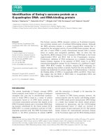
Table I. Example pedigree, marker genotypes from [1] and Q
∗
i
(bold numbers)
from (2b), in Q
i
notation (2a).
Animal Sire Dam Marker Q
∗
i
in Q
i
notation (2a)
(i) (s) (d) genotype (recombination rate: r = 0.1)
100A
1
A
1

200A
2
A
2

300A
1
A
2

412A
1
A
2
0.50 1 − 0.50 0.00 0.00
0.00 0.00 0.50 1 − 0.50
534A
1
A
1
0.50 1 − 0.50 0.00 0.00
0.00 0.00 0.90 1 − 0.90
614A
1
A
2
0.50 1 − 0.50 0.00 0.00
0.00 0.00 0.10 1 − 0.10
756A
1
A
2
0.50 1 − 0.50 0.00 0.00
0.00 0.00 0.10 1 − 0.10

D
−1
= diag(D
−1
1
, , D
−1
n
) and recursively computed B
−1
:
B
−1
1
= I
2
and B
−1
i
=







B
−1
i−1

0
−A
i
I
2







, i = 2, , n, (6)
[1] proposed efficient computational techniques using this decomposition and
a sparse storage scheme for G
−1
.
G
−1
= (B

)
−1
D
−1
B
−1
can be computed if and only if the (2×2)-matrices D
−1
i

exist for each individual i (i = 1, , n), that means all determinants det(D
i
)  0.
The example of Abdel-Azim and Freeman (see Tab. I in [1]) can be used to
demonstrate G (Fig. 1 in [1]) and G
−1
(p. 162 in [1]) for complete marker data,
linkage equilibrium and a recombination rate of 0.10 under gamete identifica-
tion by markers.
3.2. Gametes are identified by parental origin of the marker alleles
When the gametes α
1
i
, α
2
i
are identified by the parental origin of the marker
alleles, the first MQTL allele of animal i is defined as its paternal (α
1
i
=
def
α
s
i
)
and the second as its maternal allele (α
2
i
=

def
α
d
i
). Consequently (2a) becomes
Q
i
=







P(α
s
i
⇐ α
s
s
|M) P(α
s
i
⇐ α
d
s
|M) 0 0
00P(α
d

i
⇐ α
s
d
|M) P(α
d
i
⇐ α
d
d
|M)







,
and with the fact that the row sums of Q
i
are equal to 1
P(α
s
i
⇐ α
d
s
|M) = 1 − P(α
s

i
⇐ α
s
s
|M)
626 A. Tuchscherer et al.
and
P(α
d
i
⇐ α
d
d
|M) = 1 − P(α
d
i
⇐ α
s
d
|M),
i.e. only two parameters P(α
s
i
⇐ α
s
s
|M) and P(α
d
i
⇐ α

s
d
|M) are to be calculated
and therefore Q
i
reduces to
Q
∗
i
=

P(α
s
i
⇐ α
s
s
|M) P(α
d
i
⇐ α
s
d
|M)


=

Q
∗1

i
Q
∗2
i


. (2b)
Q
∗1
i
and Q
∗2
i
are known as transition probabilities in QTL analysis.
In contrast to gamete identification by markers (2a), the gametes of base
animals cannot be uniquely identified and the paternal or maternal origin of
the marker alleles of all base animals remains uncertain when (2b) is applied.
With a probability of 0.5 the first marker allele may be of paternal or maternal
origin, and the second, too. This fact creates differences in the Q
i
matrices and,
as a consequence, differences in G and its inverse if gamete identification by
parental origin is used. The same is true for heterozygous offspring of uninfor-
mative matings. For illustration, let us consider animal 5 in Table I in [1] and
Table I of this paper. Animal 5 has a marker genotype A
1
A
1
and is offspring of
animal 3 (sire, A

1
A
2
) and animal 4 (dam, A
1
A
2
). It is evident that animal 5 has
inherited A
1
from both parents. With definition (2a), this is the first allele of
the sire and the first of the dam, but because of the homozygosity, each of the
A
1
in animal 5, A
1
can be the first or the second marker allele. Thus under (2a),
Q
5
must be determined as
Q
5
=






0.500.50

0.500.50






·



















1 − rr 00
r 1 − r 00
001− rr

00r 1 − r



















=






0.45 0.05 0.45 0.05
0.45 0.05 0.45 0.05







,
where the first matrix of the product is the matrix with the probabilities of de-
scent for the marker alleles and the second is the matrix with the recombination
rate r = 0.1 in both formulas for Q
5
.
Now we use definition (2b), and the fact that the sire of 5 is base animal 3.
Hence in individual 3 A
1
can be maternal or paternal with probability 0.5. The
dam of animal 5 is no base animal. So it is clear that A
1
is the paternal allele
of the dam, and
Q
5
=






0.50.500
0010







·



















1 − rr 00
r 1 − r 00
001− rr
00r 1 − r




















=






0.50.50 0
000.90.1







Dependencies in gametic relationship matrix 627
or in (2b) notation Q
∗
5
=

0.50.9


.
The complete set of Q
∗
i
s (2b) in their Q
i
notation (2a) for Table I data in [1]
for gamete identification by parental origin can be found in Table I.
With Q
i
-notation of the Q
∗
i
the algorithm of [21] and [1] can also be ap-
plied for computing the conditional gametic relationship matrix (non-zero ele-
ments of this matrix see (E 1) and its inverse (non-zero elements of the inverse
see (E 2)).

(E 1)
(E 2)
Comparing Figure 1 in [1] and (E 1) or the matrix at page 162 in [1] and (E 2),
there are some differences in G and G
−1
.TheG-matrix [1] is of full rank and
has 128 non-zero elements, G in (E 1) is of full rank, too, but it only has 106
non-zero elements. The numbers of non-zeros in the corresponding inverses
are 74 (p. 162 in [1]) versus 58 (E 2).
With the w = Tv, model (1) can be written as MQTL genotypic effects of
model y = Xf + Zu + Zw + e, with (n × 1)-vector w of genotypic effects at
the MQTL of the n animals, E(w) = 0,Cov(w) = σ
2
w
Q
G
(n×n)
with σ
2
w
= 2σ
2
v
.It
turns out that the relation σ
2
v
· Q
G
(n×n)

= σ
2
v
· 0.5 · T
(n×2n)
G
(2n×2n)
T

(2n×n)
leads
628 A. Tuchscherer et al.
to the same conditional genotypic relationship matrix [19] (non-zero elements
in (E 3))
(E 3)
for both different conditional gametic relationship matrices Figure 1 in [1]
and (E 1). As a consequence the resulting genotypic effects w are indepen-
dent of the variant of G and the same is true for polygenic effects and the total
breeding values of all animals.
4. LINEAR DEPENDENCIES IN G AND RULES
FOR ELIMINATING THEM
As already mentioned, the recombination rate r between MQTL and the
marker may be zero for certain applications. Therefore we re-examine the ex-
ample from Table I in [1] using gamete identification by markers, but now with
a recombination rate of r = 0. The corresponding Q
i
s can be found in Table II.
With the Abdel-Azim and Freeman algorithm [1] the G-matrix can be cal-
culated, but it has dependent rows and columns (e.g. identical rows/columns 8,
12 and 14, see (E 4)).

(E 4)
The computation of G
−1
fails because of the dependencies in G. These
dependencies are indicated by det(D
i
) = 0 for individuals i = 5, 6, 7, and
consequently, D
−1
i
in (4) or (6) does not exist for these individuals. The de-
pendencies in G are caused by the configuration of Q
i
s. Problem-creating
Q
i
-matrices in the example are Q
5
, Q
6
and Q
7
in Table II. Q
6
and Q
7
imply
Dependencies in gametic relationship matrix 629
Table II. Example pedigree, marker genotypes from [1] and Q
i

(recombination rate:
r = 0.0).
For calculation
Animal Sire Dam Marker Q
i
according (2a) of (E 6), (E 7):
(i) (s) (d) genotype f
i

D
∗
i
100A
1
A
1
0 I
2
200A
2
A
2
0 I
2
300A
1
A
2
0 I
2

412A
1
A
2
0.50 0.50 0.00 0.00 0

0.50
00.5

0.00 0.00 0.50 0.50
534A
1
A
1
0.50 0.00 0.50 0.00 - -
0.50 0.00 0.50 0.00
614A
1
A
2
0.50 0.50 0.00 0.00 - 0.5
0.00 0.00 0.00 1.00
756A
1
A
2
0.50 0.50 0.00 0.00 - 0.5
0.00 0.00 0.00 1.00
that the second MQTL-alleles of individuals 6 and 7 are identical with the sec-
ond MQTL-alleles of their dams, i.e. animals 4, 6 and 7 have identical second

MQTL-alleles and this results in identical effects v
2
4
= v
2
6
= v
2
7
in model (1). Q
5
contains the information that animal 5 has received the sire’s first MQTL-allele
and the dam’s first MQTL-allele, but it is not known which of these alleles is
the first and which is the second in animal 5. Therefore Q
5
can be written as
the average Q
5
= 0.5 ·

1000
0010

+

0010
1000

, and the corresponding effects
as v

1
5
= v
2
5
= 0.5 · (v
1
3
+ v
1
4
). Hence the number of gametic effects in model (1)
can be reduced to a smaller set of different effects without dependencies in a
corresponding ‘condensed’ gametic relationship matrix G
∗
. How the config-
uration of the Q
i
s can be used in a ‘condensing’ algorithm for the gametic
effects and the computing of the ‘condensed’ gametic relationship matrix G
∗
and its inverse is outlined in detail in the following section.
Let v
∗
denote the n
∗
-dimensional vector of the n
∗
remaining components of
v and let L be a(2n × n

∗
)-dimensional matrix with row sums equal to 1 in such
a manner that v = Lv
∗
. Therewith, model (1) can be written as
y = Xf + Zu + ZT · Lv
∗
+ e,
with E(v
∗
) = 0 and Cov(v
∗
) = σ
2
v
G
∗
. The determination of the n
∗
remaining
components of v is part of the condensing algorithm. It is assumed that the Q
i
630 A. Tuchscherer et al.
matrices (2a) have already been computed for all animals and the pedigree is
ordered such that parents precede their progeny.
Let further SQ
i
=

11


· Q
i
=

SQ
1
i
SQ
2
i
SQ
3
i
SQ
4
i

define the (1 × 4)-
vector of the column sums of Q
i
.SQ
1
i
= 1 for example means that animal i has
received the first MQTL-allele of its sire and therefore SQ
2
i
= 0. If there is a
one in the first or second row of the first column of Q

i
the place of this allele
in i is the number of that row containing the one.
Define N = ((N
i,j
)), i = 1, , n; j = 1, 2a(n × 2)-dimensional integer ma-
trix with the indices of the remaining gametic effects v
∗
of n animals and
N
i
= (N
i,1
;N
i,2
)theith row of N and let n
b
be the number of base animals
at the top of the pedigree which are considered to be unrelated and non inbred,
and n
max
i−1
= max
j=1, ,i−1
k=1,2

N
j,k

.

The algorithm consists of four parts: the generation of the index matrix N,
the determination of matrix L, the calculation of the condensed gametic rela-
tionship matrix G
∗
, and finally, the computation of its inverse. It is independent
of the mode of gamete identification and can be used with Q
i
definition (2a) as
well as with Q
i
definition (2b).
First part of the algorithm: Generation of the index matrix N
For i ≤ n
b
(base animals):
N
i
= (2i − 1; 2i). (7a)
For i > n
b
(non base animals) and k, j = 1, 2:
N
i
=

























































(N
s(i),k
;N
d(i),j
);if

Q
i
(1, k) = 1 ∧ Q
i
(2, j + 2) = 1


∨

SQ
k
i
= 1 ∧ SQ
2+j
i
= 1

(N
d(i),j
;N
s(i),k
);if

Q
i
(2, k) = 1 ∧ Q
i
(1, j + 2) = 1

(N
s(i),k
;n
max
i−1
+ 1) ; if


Q
i
(1, k) = 1 ∧ SQ
2+j
i
 1, ∀j

(N
d(i),j
;n
max
i−1
+ 1) ; if

Q
i
(1, 2 + j) = 1 ∧ SQ
k
i
 1, ∀k

(n
max
i−1
+ 1; N
s(i),k
);if

Q
i

(2, k) = 1 ∧ SQ
2+j
i
 1, ∀j

(n
max
i−1
+ 1; N
d(i),j
);if

Q
i
(2, 2 + j) = 1 ∧ SQ
k
i
 1, ∀k

(n
max
i−1
+ 1; n
max
i−1
+ 2) ; if

S Q
k
i

 1, ∀k ∧ SQ
2+j
i
 1, ∀j

(7b)
where N
s(i),k
is the index of the kth MQTL-allele (k = 1, 2) of the sire s(i)
and N
d(i), j
is the index of the jth MQTL-allele ( j = 1, 2) of the dam d(i)of
Dependencies in gametic relationship matrix 631
Table III. Example from Table II – computation of index matrix N.
animal i,Q
i
(o, t)(o = 1, 2; t = 1, , 4) denotes the tth element of the oth row
in Q
i
,‘∧’/‘∨’ are the logical ‘and’/‘or’ and ‘∀’ is used in the meaning ‘for all’.
The computation of N is demonstrated with the example from Table II. Let
us consider animal 4. Animal 4 is a non-base animal. Hence (7b) must be used
to calculate N
4,1
and N
4,2
.
Q
4
=


0.50.50 0
000.50.5

and thus all four column sums of Q
4
are equal to
0.5  1, and therefore, N
4
= (n
max
3
+ 1; n
max
3
+ 2) = (7 ; 8) where n
max
3
= 6.
For the complete N see Table III.
Second part of the algorithm: Determination of the incidence matrix L
For each animal i (i = 1, , n) there are two rows in L.LetL
2i−1,t
denote
the elements of the first row and L
2i,t
(t = 1, , n
∗
) those of the second. The
following algorithm determines the non zero elements of L:

L
2i−1,t
=















Q
i
(1, k)
Q
i
(1, j)








;if

SQ
k
i
= 1 ∧ SQ
j
i
= 1

∧1  Q
i
 for







t = N
i,1
t = N
i,2
1 ; else for t = N
i,1
(8)
and
L

2i,t
=















Q
i
(2, k)
Q
i
(2, j)








;if

SQ
k
i
= 1 ∧ SQ
j
i
= 1

∧1  Q
i
 for







t = N
i,1
t = N
i,2
1 ; else for t = N
i,2
where 1  Q
i
means that no element of Q
i

equals one.
632 A. Tuchscherer et al.
For demonstration, Table II data and index matrix N from Table III are used.
The complete L-Matrix, v
∗
, v and T · v for this example are
L =








































































10000 00 000
01000 00 000
00100 00 000
00010 00 000
00001 00 000
00000 10 000
00000 01 000
00000 00 100
00000.500.5000
00000.500.5000
00000 00 010
00000 00 100
00000 00 001

00000 00 100








































































, v
∗
=












v
∗
1
.

.
.
v
∗
10












, v = Lv
∗
=









































































v
∗
1
v
∗
2
v
∗
3
v
∗
4
v
∗
5
v
∗
6
v
∗
7
v
∗
8
0.5(v
∗
5
+ v
∗
7

)
0.5(v
∗
5
+ v
∗
7
)
v
∗
9
v
∗
8
v
∗
10
v
∗
8









































































,
Tv =

































v
∗
1
+ v
∗
2
v
∗
3
+ v
∗
4
v
∗
5
+ v
∗
6
v
∗
7
+ v
∗
8
v
∗

5
+ v
∗
7
v
∗
9
+ v
∗
8
v
∗
10
+ v
∗
8

































(E 5)
Let us consider L
9,t
and L
10,t
(t = 1, , n
∗
) in more details, with the elements
of the rows L
9
and L
10

of L belonging to animal 5. From Q
5
=

0.500.50
0.500.50

follows SQ
1
i
= 1andSQ
3
i
= 1and1 Q
5
. With N
5
= (N
5,1
; N
5,2
) = (5; 7)
(see Tab. III) the non zero elements of L
9
are L
9,5
= Q
5
(1; 1) = 0.5 and with
L

9,7
= Q
5
(1; 3) = 0.5 the non zero elements of L
10
are L
10,5
= Q
5
(2; 1) = 0.5
and L
10,7
= Q
5
(2; 3) = 0.5.
Third part of the algorithm: Calculation of the condensed gametic
relationship matrix G
∗
The condensed gametic relationship matrix G
∗
with full rank n
∗
can be
computed by the use of the following generalization of the tabular method
Dependencies in gametic relationship matrix 633
of [21]: G
∗
1
= G
1

and for i = 2, , n
G
∗
i
=














































G
∗
i−1
, if N
i,1
≤ n
max
i−1
∧ N
i,2

≤ n
max
i−1
(no row/column is added)

G
∗
i−1
G
∗
i−1
A
∗k

i
A
∗k
i
G
∗
i−1
1

,ifN
i,k
> n
max
i−1
∧ N
i,j

≤ n
max
i−1
; k  j; k, j = 1, 2
(+ 1row/column)

G
∗
i−1
G
∗
i−1
A
∗
i
A
∗
i
G
∗
i−1
C
ii

,ifN
i,1
> n
max
i−1
∧ N

i,2
> n
max
i−1
(+ 2rows/column)
(9)
where A
∗
i
is a (2×n
max
i−1
)-dimensional matrix with columns N
s(i),1
,N
s(i),2
,N
d(i),1
,
N
d(i),2
being identically with the first, second, third, fourth column of Q
i
in this
order and zero elements otherwise. A
∗k
i
is the kth row of A
∗
i

,wherek = 1if
j = 2ork = 2if j = 1.
The example from Table II illustrates the computation of G
∗
(see its non-
zeroelementsin(E6))
G
∗
=

















































1.00 50 - .50 .25
-1.00 50 - .50 .25
1.00 50 - -

1.00 50 - -
1.00 50
1.00
.50 .50 1.00 - .50 .50
50 .50 1.00 - -
.50 .50 50 - 1.00 .25
.25 .25 - - .50 - .50 - .25 1.00

















































(E 6)
and more detailed G
∗
i
for animal i = 7.

G
∗
6
is the matrix with the first 9 rows and columns in (E 6) with rank(G
∗
6
) =
n
max
6
= 9. From Table III we get N
7
= (N
7,1
;N
7,2
) = (10; 8) for animal 7,
N
s(7)
= N
5
= (5; 7) for its sire and N
d(7)
= N
6
= (9; 8) for its dam. N
7,1
=
10 > n
max

6
= 9andN
7,2
= 8 ≤ n
max
6
= 9 implies that the first row of A
∗
7
must
be used, containing the elements (0.5 0.5 0 0) of the first row of Q
7
(Tab. II)
at the places 5, 7, 9, 8: A
∗1
7
=

00000.500.500

. Therefore A
∗1
7
G
∗
6
re-
sults in

.25 .25 .00 .00 .50 .00 .50 .00 .25


and G
∗
7
=







G
∗
6
G
∗
6
A
∗1
7
A
∗1
7
G
∗
6
1








= G
∗
(see (E 6)).
634 A. Tuchscherer et al.
Fourth part of the algorithm: Computation of the inverse of the condensed
gametic relationship matrix G
∗
The inverse G
∗−1
of the condensed gametic relationship matrix G
∗
can be
determined by generalization of the tabular method of [21] in an analogous
way: G
∗−1
1
= G
−1
1
and for i = 2, , n
G
∗−1
i
=









































G
∗−1
i−1
, if N
i,1
≤ n
max
i−1
∧ N
i,2
≤ n
max
i−1

G
∗−1
i−1
0
0 0

+








1
d
∗
i
A
∗k
i
A
∗k
i
−
1
d
∗
i
A
∗k
i
−
1
d
∗
i
A

∗k
i
1
d
∗
i







, if N
i,k
> n
max
i−1
∧ N
i,j
≤ n
max
i−1
;
k  j; k, j = 1, 2

G
∗−1
i−1
0

0 0

+

A
∗
i
D
∗−1
i
A
∗
i
−A
∗
i
D
∗−1
i
−D
∗−1
i
A
∗
i
D
∗−1
i

, if N

i,1
> n
max
i−1
∧ N
i,2
> n
max
i−1
(10)
where d
∗
i
= (1 − A
∗k
i
G
∗
i−1
A
∗k
i
) if one row and column is added and
D
∗
i
= (C
ii
− A
∗

i
G
∗
i−1
A
∗
i
) if two rows and columns are added. Calculation
of d
∗
i
and D
∗
i
can be simplified by using d
∗
i
= (1 − Q
k
i

G
i
Q
k
i
)and
D
∗
i

= (C
ii
− Q
i

G
i
Q

i
), where Q
k
i
is the kth row of Q
i
and

G
i
=







G
s(i)
G

s(i)d(i)
G
d(i)s(i)
G
d(i)







,
with
G
s(i)d(i)
=







G
∗
i−1
(N
s(i),1
;N

d(i),1
)G
∗
i−1
(N
s(i),1
;N
d(i),2
)
G
∗
i−1
(N
s(i),2
;N
d(i),1
)G
∗
i−1
(N
s(i),2
;N
d(i),2
)








= G

d(i)s(i)
,
G
s(i)
=

1f
s(i)
f
s(i)
1

, f
s(i)
= G
∗
i−1
(N
s(i),1
;N
s(i),2
), G
d(i)
=

1f
d(i)

f
d(i)
1

,
f
d(i)
= G
∗
i−1
(N
d(i),1
;N
d(i),2
)andG
∗
i−1
(o; t)isthetth element in the oth row of
G
∗
i−1
.
We continue with animal 7 for illustration of (10). With G
∗−1
6
we only have
to compute d
∗
7
to get G

∗−1
7
= G
∗−1
(see (E 7) for non-zero elements of the
Dependencies in gametic relationship matrix 635
inverse G
∗−1
) with A
∗1
7
=

00000.500.500

from above.
G
∗−1
=


















































2.00 1.00 −1.00 - −1.00 -
1.00 2.00 −1.00 - −1.00 -
1.50 .50 - - - −1.00 - -
50 1.50 - - - −1.00 - -
1.50 - .50 - - −1.00
1.00
−1.00 −1.00 - - .50 - 2.50 - - −1.00
−1.00 −1.00 - - - 2.00 - -
−1.00 −1.00 2.00 -
−1.00 - −1.00 - - 2.00


















































(E 7)
with
f
s(7)
= G
∗
6
(N
s(7),1
;N
s(7),2
) = G
∗
6
(5, 7) = 0,
f
d(7)
= G
∗
6
(N
d(7),1
;N
d(7),2
) = G

∗
6
(9; 8) = 0
and
G
s(7)d(7)
=







G
∗
6
(N
s(7),1
;N
d(7),1
)G
∗
6
(N
s(7),1
;N
d(7),2
)
G

∗
6
(N
s(7),2
;N
d(7),1
)G
∗
6
(N
s(7),2
;N
d(7),2
)







=







G

∗
6
(5; 9) G
∗
6
(5; 8)
G
∗
6
(7; 9) G
∗
6
(7; 8)







=







00
0.50








and the first row (k = 1) of Q
7
(Tab. II) is d
∗
7
= (1−Q
1
7

G
7
Q
1

7
) = (1−0.5) = 0.5.
Thus −
1
d
∗
7
A
∗1

7
= −2 · A
∗1
7
is equal to

0000−10−100

(see (E 7)).
Finally, it is straightforward to verify that LG
∗
L

= G,whereL is from
(E 5), G
∗
from (E 6) and G from (E 4).
Decomposition of G
∗
from (9) into G
∗
= B
∗
D
∗
B
∗

can be done in an analogy
to (4) with D

∗
= diag(

D
∗
1
, ,

D
∗
n
), where

D
∗
i
=


















− , if N
i,1
≤ n
max
i−1
∧ N
i,2
≤ n
max
i−1
(no row/column is added)
d
∗
i
, if N
i,k
> n
max
i−1
∧ N
i, j
≤ n
max
i−1
; k  j; k, j = 1, 2(+ 1row/column)
D

∗
i
, if N
i,1
> n
max
i−1
∧ N
i,2
> n
max
i−1
(+ 2rows/column)
(11)
636 A. Tuchscherer et al.
and d
∗
i
and D
∗
i
are from (10) recursively calculated B
∗
: B
∗
1
= I
2
and for i =
2, , n:

B
∗
i
=




































B
∗
i−1
,ifN
i,1
≤ n
max
i−1
∧ N
i,2
≤ n
max
i−1
(no row/column is added)

B
∗
i−1
0
A
∗k

i
B
∗
i−1
1

,ifN
i,k
> n
max
i−1
∧ N
i,j
≤ n
max
i−1
; k  j; k, j = 1, 2
(+ 1row/column)

B
∗
i−1
0
A
∗
i
B
∗
i−1
I

2

,ifN
i,1
> n
max
i−1
∧ N
i,2
> n
max
i−1
(+ 2rows/columns)
(12)
Consequently, the inverse of the condensed gametic relationship matrix G
∗
can
be calculated as G
∗−1
= (B
∗

)
−1
D
∗−1
B
∗−1
, with D
∗−1

= diag(

D
∗−1
1
, ,

D
∗−1
n
)
and recursively determined B
∗−1
: B
∗−1
1
= I
2
and for i = 2, , n
B
∗−1
i
=


































B
∗−1
i−1
,ifN

i,1
≤ n
max
i−1
∧ N
i,2
≤ n
max
i−1
(no row/column is added)

B
∗−1
i−1
0
−A
∗k
i
1

,ifN
i,k
> n
max
i−1
∧ N
i,j
≤ n
max
i−1

; k  j; k, j = 1, 2
(+ 1row/column)

B
∗−1
i−1
0
−A
∗
i
I
2

,ifN
i,1
> n
max
i−1
∧ N
i,2
> n
max
i−1
(+ 2rows/columns)
(13)
in analogy to (5).
With w = Tv, v = Lv
∗
, the relation Q
G

= 0.5 · TGT

= 0.5 · T(LG
∗
L

)T

between conditional genotypic relationship matrix Q
G
and conditional gametic
relationship matrices G and G
∗
, it is easy to verify that G
∗
from (E 6) and G
from (E 4) result in the same conditional genotypic relationship matrix
Q
G
=
































1.000 - - 0.500 0.500 0.500 0.250
-1.000 - 0.500 - 0.500 0.500
1.000 - 0.500 - 0.250
0.500 0.500 - 1.000 0.500 0.750 0.750
0.500 - 0.500 0.500 1.000 0.250 0.500
0.500 0.500 - 0.750 0.250 1.000 0.625
0.250 0.500 0.250 0.750 0.500 0.625 1.000
































· (E 8)

Again, we consider the situation that the gametes α
1
i
, α
2
i
are identified by
parental origin for Table II data and calculate Q
∗
i
according to (2b). The Q
∗
i
sfor
Dependencies in gametic relationship matrix 637
the non-base animals are Q
∗
4
=

0.50.5


, Q
∗
5
=

0.51.0



, Q
∗
6
=

0.50.0


and Q
∗
7
=

0.50.0


. Applying the condensing algorithm for this data, the
condensed gametic relationship matrix G
∗
(see (E 9) for non-zero elements)























































1.00 50 - - .50 .25
-1.00 50 - - .50 .25
1.00 50
1.00 50
1.00 50 - .25
1.00 - - .50 - .25
.50 .50 1.00 - - .50 .50
50 .50 1.00
50 .50 - - 1.00 - .50
.50 .50 50 - - 1.00 .25
.25 .25 - - .25 .25 .50 - .50 .25 1.00























































(E 9)
and its inverse G
∗−1
(see (E 10) for non-zero elements)























































2.00 1.00 −1.00 - - −1.00 -
1.00 2.00 −1.00 - - −1.00 -
1.50 .50 - - - −1.00
50 1.50 - - - −1.00
1.50 .50 - - −1.00 - -
50 1.50 - - −1.00 - -
−1.00 −1.00 2.50 - .50 - −1.00
−1.00 −1.00 - - - 2.00
−1.00 −1.00 .50 - 2.50 - −1.00
−1.00 −1.00 2.00 -
−1.00 - −1.00 - 2.00























































(E 10)
can be calculated recursively. In contrast to (E 5) (10 remaining effects) there
are now 11 effects left. The differences in the condensed gametic relationship
matrices ((E 6) vs. (E 9)) and their inverses ((E 7) vs. (E 10)) are evident. G
∗
in (E 6) is of rank 10 and has 34 non-zero elements, G
∗
in (E 9) is of rank 11
and has 43 non-zero elements. The corresponding inverses are of rank 10 with
32 non-zeros (E 7) versus rank 11 with 39 non-zero elements (E 10). But again
the matrices of (E 6) and (E 9) result in the identical genotypic relationship

matrix (E 8), which can easily be verified. This means that the number and
size of estimates of gametic MQTL effects depend on the mode of gamete
identification, but the sum of these effects remains unaffected for each animal.
638 A. Tuchscherer et al.
5. DISCUSSION
Gamete identification by parental origin and gamete identification by mark-
ers have already been used earlier in the literature without a clear distinc-
tion [1, 2, 14, 21]. In this article it was shown for the first time, at least to the
authors’ knowledge, that both identification methods result in different condi-
tional gametic relationship matrices and different estimates of gametic effects
in a MA-BLUP model. It could, however, be demonstrated that the MA-BLUP
breeding value – the estimated sum of QTL-gamete effects and the polygenic
effect – remain the same irrespective of the method of gamete identification.
A practical advantage of identification by parental origin is that both the
sire-block and the dam-block of the Q
i
-matrices (2a) can each be represented
by a single number, namely the probability that the paternal allele of the sire
and the dam have been transmitted to the descendant, respectively. The rea-
son for this is that each block (sire and dam) of the Q
i
-matrices has only two
non-zero entries which sum up to one, if the Q
i
-matrices reflect gamete identi-
fication by parental origin. The alternative mode of gamete identification needs
three probabilities for each block, because the number of non-zero entries per
block (again summing up to one) is four when gamete identification is done by
marker. It may be worthwhile to store Q
i

-matrices for all animals additionally
to marker raw data as an essence of marker information and intermediate result
in computing the G matrix and its inverse and also for other purposes as e.g.
the computation of measures of marker information content. Though six num-
bers per animal will not be prohibitive to store even with tens of thousands of
animals, identification by parental origin needs only two and is therefore easier
to administer.
The genotypic relationship matrix Q
G
in the MQTL genotypic effect model
may either be determined by deterministic methods [1, 2, 9, 13, 21] or by
Markov chain Monte Carlo (MCMC) [5, 12, 16–18, 20] and their advantages
and disadvantages have been investigated by several authors [11, 13]. MCMC
has been implemented in the LOKI program [6] in order to compute Q
G
by
MCMC, but currently it cannot be used to compute G for a MQTL allelic ef-
fects model. Though not primarily designed for this purpose SimWalk2 [15]
can be employed to achieve this goal: it reports MCMC estimates of all 15
detailed identity state probabilities [4] between any pair of animals in the pedi-
gree. Q
i
matrices can be derived from the SimWalk2 output implicitly using
gamete identification by parental origin. This follows from the definition of
identity states in SimWalk2 software [15].
The MA-BLUP breeding value of each animal in (1) equals the sum of the
MQTL genotypic effect and the polygenic effect. Thus it would be sufficient to
Dependencies in gametic relationship matrix 639
use a MQTL genotypic effects model and to save one equation per genotyped
animal. Since the MQTL genotypic effect is the sum of the first and the second

MQTL allele effects, one positive and one negative gametic effect may give rise
to the same genotypic effect as two gametic effects of average size. It would be
interesting for breeders to know how an MQTL genotypic effect is composed
and therefore it is desirable to have estimates of the available gametic effects.
A conclusion of the considerations above is, that a certain mode of gamete
identification has to be chosen. It may be more natural to animal breeders to
think in pedigrees and parental origin rather than in marker haplotypes and
therefore gamete identification by parental origin may be preferred for this
purpose.
It has been proposed by [11] to estimate MQTL genotypic effects w and to
transform these into allelic effects v. If such a transformation exists, it would
have to be specific for a certain definition of v, i.e. it would depend on the mode
of gamete identification. The conclusion of [11] that v = 0.5 · GT

(Q
G
(n×n)
)
−1
w
follows from Tv = w = TGT

(TGT

)
−1
w = 0.5·TGT

(Q
G

(n×n)
)
−1
w is however
not possible, because a left-inverse, say T
(left)−
,ofT with T
(left)−
(2n×n)
T
(n×2n)
= I
2n
does not exist. For the proof we only have to consider the first two elements of
the first row of T
(left)−
(2n×n)
T
(n×2n)
T
(left)−
(2n×n)
T
(n×2n)
=













t
1,1
t
1,2
··· t
1,n
.
.
.
.
.
.
.
.
.
.
.
.
t
2n,1
t
2n,2
··· t

2n,n






























1100··· 00
00
11··· 00
.
.
.
.
.
.
.
.
.
.
.
.
.
.
.
.
.
.
.
.
.
00
00··· 11


















=







t
1,1
t
1,1
···
.
.
.
.

.
.
.
.
.







 I
2n
,
where t
1,1
cannot take the values 1 and 0 at the same time, and consequently,
T
(left)−
(2n×n)
T
(n×2n)
never equals the identity matrix.
Both modes of gamete identification fail for some animals. The gametes of
homozygous individuals (both base and non-base) cannot be distinguished by
markers. On the contrary, gamete identification by parental origin fails in all
founders and in all non-founders from non-informative matings, where from
marker analysis it cannot be deduced whether the marker was inherited from
the dam or from the sire. As the number of markers is increased, the probabil-

ity for a mating to be non-informative for all markers as well as the probability
for an individual to be homozygous at all marker loci becomes smaller and
smaller. Multiple markers will therefore help to identify nearly all gametes un-
equivocally. This is, however, not true for founder animals, when gamete iden-
tification is done by parental origin. This problem can, however, be resolved
by identifying founder gametes by markers and by arbitrarily denoting one of
640 A. Tuchscherer et al.
both gametes of each founder animal as maternal and the other as paternal.
By applying this rule to the example pedigree [1] it can be shown that a third
variant of a conditional gametic relationship matrix results and differs from
the two others demonstrated above (data not shown), but again transforms to
the same Q
G
-matrix and, consequently, leads to the same MA-BLUP breeding
values.
Gamete identification by marker may be of interest in applications where
the intention is to test a certain polymorphism for linkage disequilibrium with
a QTL. With two alleles and in using this polymorphism for gamete identifica-
tion, all gametes with allele 1 are treated as the first and all gametes with allele
2 as the second gamete of heterozygous animals. The expectation is that, if the
polymorphism is in strong linkage disequilibrium with the QTL, differences
between the first and the second gametic effect of heterozygotes will exhibit
the same sign and roughly the same size, provided there is a sufficient accuracy
of both gametic estimates.
A reduction of the size of the conditional gametic relationship matrix has
already been proposed by [10]: parents and offspring sharing the same marker
haplotype were treated as sharing the same QTL allele, by assuming a zero
probability of double recombinations. In these cases the same gametic QTL
effect was assigned to the parent and the offspring. When the offspring has
received a recombinant marker haplotype a new gametic QTL effect was de-

fined as the average of both gametes of the parent animal. Treating these two
gametes as parents of the new gamete allows to set up a pedigree of gametic ef-
fects and to compute the conditional gametic relationship matrix and its inverse
simply by applying the Henderson rules [7,8]. The condensing algorithm will,
of course, lead to identical results, if desired: sire- and dam-blocks of progeny
with non-recombinant parental haplotypes have to carry zeros and ones only,
and in the recombinant case the corresponding sire- and dam-blocks are as-
sembled by fifty-percent transition probabilities as in the case without mark-
ers. The Meuwissen and Goddard proposal [10] therefore combines a special
case of the condensing algorithm with gamete identification by parental origin.
Assuming the QTL in the middle of a certain marker interval and rounding the
QTL-transition probabilities to either one or zero if they are closer to these
values as a predefined threshold, e.g. 0.02, will give the same results as in [10]
for those animals which are informative at the markers flanking this particu-
lar interval. For the other animals information from markers more remote and
asymmetrically distributed around the QTL’s assumed home interval may be
available. In these cases the probability of double recombinations may be too
high to be neglected and, furthermore, the assumption of an equal transmission
Dependencies in gametic relationship matrix 641
probability of the first and second parental allele may be unrealistic in the light
of the markers transmitted. These animals can easily be combined with the
former group by maintaining the original transition probabilities in the Q
i
-
matrices without rounding and then applying the condensing algorithm to all
pedigree members in the same way, no matter of previous rounding or not.
In conclusion, the condensing algorithm is a generalization of the Abdel-
Azim and Freeman algorithm [1] for computing the conditional gametic rela-
tionship matrix and its inverse. Although suggested before by other authors,
computing this inverse cannot be avoided if estimates of gametic QTL effects

are desired.
The condensing algorithm can be applied to different modes of gamete iden-
tification, situations with and without markers including X-linkage, clones and
haplodiploid pedigrees. Treatment of haplotypes according to the proposals
of [10] are covered as a special case and can be combined with exact treatment
of more remote marker information.
ACKNOWLEDGEMENTS
The authors would like to thank Dr. Fritz Reinhardt and Dr. Hauke Thom-
sen (Vereinigte Informationssysteme Tierhaltung w. V. Verden, Germany), Dr.
Jörn Bennewitz (Institut für Tierzucht und Tierhaltung, Christian-Albrechts-
Universität Kiel, Germany) for their helpful discussion and Dr. Gertraude
Freyer for useful hints on SimWalk2 software.
REFERENCES
[1] Abdel-Azim G., Freeman A.E., A rapid method for computing the inverse of
the gametic covariance matrix between relatives for a marked Quantitative Trait
Locus, Genet. Sel. Evol. 33 (2001) 153–173.
[2] Fernando R.L., Grossman M., Marker-assisted selection using best linear unbi-
ased prediction, Genet. Sel. Evol. 21 (1989) 467–477.
[3] Georges M., Recent progress in livestock genomics and potential impact on
breeding programs, Theriogenology 55 (2001) 15–21.
[4] Gillois M., La relation d’identité en génétique, Thèse Faculté des Sciences de
Paris (1964).
[5] Grignola F.G., Hoeschele I., Tier B., Mapping quantitative trait loci via residual
maximum likelihood, I. Methodology, Genet. Sel. Evol. 28 (1996) 479–490.
[6] Heath S.C., Markov chain Monte Carlo segregation and linkage analysis for oli-
gogenic models, Am. J. Hum. Genet. 61 (1997) 748–760.
[7] Henderson C.R., Best linear unbiased estimation and prediction under a selection
model, Biometrics 31 (1975) 423–439.
642 A. Tuchscherer et al.
[8] Henderson C.R., A simple method for computing the inverse of a numerator

relationship matrix used in prediction of breeding values, Biometrics 32 (1976)
69–83.
[9] Knott S.A., Elsen J.M., Haley C.S., Methods for multiple marker mapping of
quantitative trait loci in half-sib populations, Theor. Appl. Genet. 93 (1996)
71–80.
[10] Meuwissen T.H.E., Goddard M.E., The use of marker-haplotypes in animal
breeding schemes, Genet. Sel. Evol. 28 (1996) 161–176.
[11] Nagamine Y., Knott S.A., Visscher P.M., Haley C.S., Simple deterministic
identity-by-descent coefficients and estimation of QTL allelic effects in full and
half sibs, Genet. Res. Camb. 80 (2002) 237–243.
[12] Pérez-Enciso M., Varona L., Rothschild M.F., Computation of identity by de-
scent probabilities conditional on DNA markers via a Monte Carlo Markov chain
method, Genet. Sel. Evol. 32 (2000) 467–482.
[13] Pong-Wong R., George A.W., Woolliams J.A., Haley C.S., A simple and rapid
method for calculating identity-by-descent matrices using multiple markers,
Genet. Sel. Evol. 33 (2001) 453–471.
[14] Schaeffer L.R., Kennedy B.W., Gibson J.P., The inverse of the gametic relation-
ship matrix, J. Dairy Sci. 72 (1989) 1266–1272.
[15] Sobel E., Lange K., Descent graphs in pedigree analysis: applications to hap-
plotyping, location scores, and marker-sharing statistics, Am. J. Hum. Genet. 58
(1996) 1323–1337.
[16] Thompson E.A., Monte Carlo likelihood in genetic mapping, Stat. Sci. 9 (1994)
355–366.
[17] Thompson E.A., Inferring gene ancestry: estimating gene descent, Int. Stat. Rev.
66 (1998) 29–40.
[18] Thompson E.A., Heath S.C., Estimation of conditional multilocus gene identity
among relatives, in: Seiller-Moseiwitch F., Donelly P., Watermann M. (Eds.),
Statistics in Molecular Biology, Springer-Verlag IMS lecture note series, New
York, 1999.
[19] van Arendonk J.A.M., Tier B., Kinghorn B.P., Use of multiple genetic markers

in prediction of breeding values, Genetics 137 (1994) 319–329.
[20] Visscher P.M., Haley C.S., Heath S.C., Muir W.J., Blackwood DHR Detecting
QTLs for uni- and bipolar disorder using a variance component method, Psych.
Genet. 9 (1999) 75–84.
[21] Wang T., Fernando R.L., van der Beek S., Grossman M., van Arendonk J.A.M.,
Covariance between relatives for a marked quantitative trait locus, Genet. Sel.
Evol. 27 (1995) 251–274.