Báo cáo sinh học: "Analysis of a simulated microarray dataset: Comparison of methods for data normalisation and detection of differential expression (Open Access publication)" pps
Bạn đang xem bản rút gọn của tài liệu. Xem và tải ngay bản đầy đủ của tài liệu tại đây (796.66 KB, 15 trang )
Genet. Sel. Evol. 39 (2007) 669–683 Available online at:
c
INRA, EDP Sciences, 2007 www.gse-journal.org
DOI: 10.1051/gse:2007031
Original article
Analysis of a simulated microarray dataset:
Comparison of methods for
data normalisation and detection
of differential expression
(Open Access publicati on)
Michael Wat s o n
a∗
, Mónica P
´
erez
-Alegre
b
, Michael Denis
B
aron
c
, Céline Delmas
d
, Peter Dov
ˇ
c
e
,MylèneDuval
d
,
Jean-Louis F
oulley
f
, Juan José Garrido-Pav
´
on
b
,Ina
H
ulsegge
g
,FlorenceJaffr
´
ezic
f
, Ángeles Jim
´
enez-Mar
´
in
b
,
Miha L
av r i
ˇ
c
e
,Kim-AnhL
ˆ
e
Cao
h
, Guillemette Marot
f
, Daphné
M
ouzaki
h
, Marco H. Pool
c
, Christèle Robert-Grani
´
e
d
, Magali
S
an Cristob al
d
, Gwenola Tosser-Klopp
d
,David
W
addington
h
,Dirk-Jande Koning
h
a
Institute for Animal Health, Compton, UK (IAH_C)
b
University of Cordoba, Cordoba, Spain (CDB)
c
Institute for Animal Health, Pirbright, UK (IAH_P)
d
INRA, Castanet-Tolosan, France (INRA_T)
e
University of Ljubljana, Slovenia (SLN)
f
INRA, Jouy-en-Josas, France (INRA_J)
g
Animal Sciences Group Wageningen UR, Lelystad, NL (IDL)
h
Roslin Institute, Roslin, UK (ROSLIN)
(Received 10 May 2007; accepted 10 July 2007)
Abstract – Microarrays allow researchers to measure the expression of thousands of genes in
a single experiment. Before statistical comparisons can be made, the data must be assessed
for quality and normalisation procedures must be applied, of which many have been proposed.
Methods of comparing the normalised data are also abundant, and no clear consensus has yet
been reached. The purpose of this paper was to compare those methods used by the EADGENE
network on a very noisy simulated data set. With the aprioriknowledge of which genes are
differentially expressed, it is possible to compare the success of each approach quantitatively.
Use of an intensity-dependent normalisation procedure was common, as was correction for
∗
Corresponding author:
Institute for Animal Health Informatic groups, Compton Laboratory, Compton RG20 7 NN
Newbury Bershive, UK.
Article published by EDP Sciences and available at
or />670 M. Watson et al.
multiple testing. Most variety in performance resulted from differing approaches to data quality
and the use of different statistical tests. Very few of the methods used any kind of background
correction. A number of approaches achieved a success rate of 95% or above, with relatively
small numbers of false positives and negatives. Applying stringent spot selection criteria and
elimination of data did not improve the false positive rate and greatly increased the false negative
rate. However, most approaches performed well, and it is encouraging that widely available
techniques can achieve such good results on a very noisy data set.
gene expression / two colour microarray / simulation / statistical analysis
1. INTRODUCTION
Microarrays have become a standard tool for the exploration of global gene
expression changes at the cellular level, allowing researchers to measure the
expression of thousands of genes in a single experiment [16]. The hypothesis
underlying the approach is that the measured intensity for each gene on the ar-
ray is proportional to its relative expression. Thus, biologically relevant differ-
ences, changes and patterns may be elucidated by applying statistical methods
to compare different biological states for each gene. However, before com-
parisons can be made, a number of normalisation steps should be taken in
order to remove systematic errors and ensure the gene expression measure-
ments are comparable across arrays [15]. There is no clear consensus in the
community about which methods to use, though several reviews have been
published [8, 12]. After normalisation and statistical tests have been applied,
there is an additional problem of multiple testing. Due to the high number of
tests taking place (many thousands in most cases), the resulting P-values must
be adjusted in order to control or estimate the error rate (see [14] for a review).
The aim of this paper was to summarise and compare the many methods
used throughout the EADGENE network () for mi-
croarray analysis, and compare the results, with the final aim of producing
a guide for best practice within the network [4]. This paper describes a variety
of methods applied to a simulated data set produced by the SIMAGE pack-
age [1]. The data set is a simple comparison of two biological states on ten
arrays, with dye-balance. A number of data quality, normalisation and analysis
steps were used in various combinations, with differing results.
1.1. The data
SIMAGE takes a number of parameters, which were produced using a slide
from the real data set as an example [4]. The input values that were used for
the current simulations are given in Table I. The simulated data consists of
Data normalisation of gene expression analysis 671
ten microarrays each of which represent a direct comparison between differ-
ent biological samples from situation A and B with a dye balance. SIMAGE
assumes a common variance for all genes, something which may not be true
for real data. Each slide had 2400 genes in duplicate, with 48 blocks arranged
in 12 rows and 4 columns (100 spots per block). Each block was “printed”
with a unique print tip. In the simulated data 624 genes were differentially
expressed: 264 were up-regulated from A to B while 360 were down regu-
lated. This information was only provided to the participants at the end of the
workshop. The simulated data are available upon request from D.J. de Koning
().
The data are very noisy with high levels of technical bias and thus provided
a serious challenge for the various analysis methods that were applied. Many
spots reported background higher than foreground, and others reported a zero
foreground signal. Image plots of the arrays showed clear spatial biases in both
foreground and background intensities (Fig. 1). Spots, scratches and stripes of
background variation are clearly visible, which have been simulated using the
“hair” and “disc” parameters of SIMAGE.
All of the slides show a clear relationship between M (log ratio) and A
(average log intensity), and the plots in Figure 2 are exemplars. Slides 3, 5,
6, 7, 9 and 10 displayed a negative relationship between M and A, whilst the
others displayed a positive relationship. Slides 6 and 9 showed an obvious non-
linear relationship between M and A, but only slide 2 levels off with higher
values of A. Finally, Figure 3 shows the range of M values for each array
under three different normalisation strategies: none (Fig. 3a), LOESS (Fig. 3b)
and LOESS followed by scale normalisation between arrays (Fig. 3c) [17,19].
It can be seen that before normalisation there is a clear difference in both the
median log ratios and the range of log ratios across slides.
This data set was subject to a total of 12 different analysis methods, encom-
passing a variety of techniques for assessing data quality, normalisation and
detecting differential expression. These methods are described in detail and
the results of each presented and compared. The results are then discussed in
relation to the best methods to use for analysing extremely noisy microarray
data.
2. MATERIALS AND METHODS
2.1. Preprocessing and normalisation procedures
A variety of pre-processing and normalisation procedures were used in
combination with the twelve different methods, and these are summarised in
672 M. Watson et al.
Table I. Settings for Simage simulation software.
Array number of grid rows 12
Array number of grid columns 4
Number of spots in a grid row 10
Number of spots in a grid column 10
Number of spot pins 48
Number of technical replicates 2
Number of genes 0
Number of slides 10
Perform dye swaps yes
Gene expression filter yes
Reset gene filter for each slide no
Mean signal 10.33
Change in log
2
ratio due to upregulation 1.07
Change in log
2
ratio due to downregulation –1.26
Variance of gene expression 2.7
% of upregulated genes 15
% of downregulated genes 11
Correlation between channels 1
Dye filter yes
Reset dye filter for each slide yes
Channel variation 0.2
Gene × Dye 0
Error filter yes
Reset error filter for each slide yes
Random noise standard deviation 0.62
Tail behaviour in the MA plot 0.108
Non-linearity filter yes
Reset non-linearity filter for each slide yes
Non-linearity parameter curvature 0.2
Non-linearity parameter tilt 4.5
Non-linearity from scanner filter yes
Reset non-linearity scanner filter for each slide yes
Scanning device bias 0.04
Spotpin deviation filter yes
Reset spotpin filter for each slide no
Spotpin variation 0.32
Background filter yes
Reset background filter for each slide yes
Number of background densities 5
Mean standard deviation per background density 0.2
Maximum of the background signal relative to the non-background signals 50
Standard deviation of the random noise for the background signals 0.1
Background gradient filter no
Reset gradient filter for each slide yes
Maximum slope of the linear tilt 700
Missing values filter yes
Reset missing spots filter for each slide yes
Number of hairs 3
Maximum length of hair 20
Number of discs 4
Average radius disc 10
Number of missing spots 50
Data normalisation of gene expression analysis 673
Figure 1. Example background plots. The top two images show the background for
Cy5 and Cy3 in slide 9, and the bottom two images show the same for slide 10.
Table II. Only one method, IDL1, chose to perform background correction.
Some methods chose to eliminate spots, or give them zero weighting, depend-
ing on particular data quality statistics; these included having foreground less
than a given multiple of background, saturated spots and spots whose inten-
sity was zero. IAH_P1 and IDL1 also removed entire slides considered to have
poor data quality. Both IAH_P and IDL submitted two approaches, one based
on strict quality control and normalisation, and the second less strict.
Most approaches applied a version of LOWESS or LOESS normalisation,
either globally or per print-tip [19]. This is in recognition of the clear rela-
tionship between M and A. Only ROSLIN (assessed normalisation by row and
674 M. Watson et al.
Figure 2. MA-plots of slides 1, 5 and 6. These slides are examples of the three pat-
terns displayed by the simulated data in the MA-space: positive correlation, negative
correlation and a more pronounced non-linear correlation.
Figure 3. Boxplots of M values (log
2
(cy5/cy3)) across the 10 arrays for three nor-
malisation strategies: (A) Unnormalised data, (B) LOESS normalised data, and (C)
LOESS followed by scale normalised data.
column and found not needed) and INRA_J (correction by block) applied any
further spatial normalisation. SLN1 and SLN2 applied median normalisation.
Finally, only IDL attempted any correction between arrays by fitting a mono-
tonic spline in MA-space to correct for heterogeneous variance. The smooth-
ing function was fitted to the absolute log ratios (M-values) across the log
mean intensities (A-values), and corrected for. This ensured that the variance
in M values was consistent across arrays.
Data normalisation of gene expression analysis 675
Table II. Summary of the 12 methods used for analysing the simulated data. “Anal-
ysis name” is the name of the analysis method, “Data quality procedures” describe
the methods approach to data quality, “Background correction” whether background
correction was carried out, “Normalisation” describes the normalisation method and
“Differential expression” describes the method’s approach to finding differentially ex-
pressed genes.
Analysis
name
Data quality
procedures
Background
correction
Normalisation Differential
expression
IAH_P1 Eliminated spots with net
intensity < 0.
Slides 5, 6 and 9 deleted
No global LOWESS Limma;
FDR correction
IAH_P2 Slides 5, 6 and 9 deleted No global LOWESS Limma;
FDR correction
IDL1 Eliminated
• control spots
• null spots
• oversaturated spots
• values < 3* SD bgnd. printtip LOWESS; Limma;
Slides 5 and 7 deleted Yes monotonic spline correction FDR correction
IDL2 No global LOWESS;
monotonic spline correction
Limma;
FDR correction
INRA_J Spots == zero removed No LOWESS;
median normalisation by block
structural mixed model;
FDR correction
INRA_T1 Spots == zero removed No global LOWESS Student statistic;
FDR correction
INRA_T2 Spots == zero removed No global LOWESS Student statistic;
Duval correction
INRA_T3 Spots == zero removed No global LOWESS Student statistic;
Bordes correction
ROSLIN Spots == zero removed No printtip LOWESS;
row-column normalisation
Limma;
FDR correction
SLN2 Only use data where FG >
1.5* BG
No median normalisation Anova (Orange)
CDB Elimination of spots with
huge M-values
No printtip LOWESS fold change cut-off
(+/–0.9)
SLN1 Excluded BG > FG No median normalisation Anova (GeneSpring)
2.2. Methods for finding differentially expressed genes
Table II summarises the twelve methods used for analysing the simulated
data set. Most variation in the methods came from the area of quality control,
with different groups excluding different genes/arrays based on a wide variety
of criteria, and correction for multiple testing.
Almost all analysis methods used some variation of linear modelling fol-
lowed by correction for multiple testing to find differentially expressed genes.
The most common of those used was the limma package, which adjusts the
t-statistics by empirical Bayes shrinkage of the residual standard errors to-
ward a common value (near to the median) [17]. IAH_P and ROSLIN fitted
676 M. Watson et al.
acoefficient for the dye-effect for each gene, which was found to be non-
significant. IAH_P also adjusted the default estimated proportion of differen-
tially regulated genes in the eBayes procedure to 0.2 once it became clear that
a high percentage of the genes in the dataset were differentially regulated. This
ensured a good estimate of the posterior probability of differential expression.
Of those that did not use limma, both SLV and SLN2 used an ANOVA
approach, implemented in GeneSpring [9] and Orange [5] respectively.
INRA_J used a structural mixed model, more completely described in Jaffrézic
et al. [11]. CDB employed a cut-off value for the mean log ratio to define the
proportion of differentially expressed genes [10, 18]. INRA_T presented three
methods all based on a classic Student statistic and an empirical variance cal-
culated for each gene, but with the P-values adjusted according to Benjamini
and Hochberg [2], Duval et al. (partial sums of ordered t-statistics) [6, 7] and
Bordes et al. (mixture of central and non-central t-statistics) [3]. Apart from
INRA_T, those methods that corrected P-values for multiple testing did so us-
ing the FDR as described by Benjamini and Hochberg [2]. All corrections for
multiple testing were carried out at the 5% level.
All methods treated the 10 arrays as separate, biological replicates apart
from ROSLIN, who treated the dye-swaps as technical replicates. The INRA_J
and the three INRA_T methods treated replicate spots as independent mea-
sures, resulting in up to 20 values per gene, whereas the other methods aver-
aged over replicate spots. INRA_T reported that preliminary analysis showed
very few differences between treating duplicates as independent or by averag-
ing them.
3. RESULTS
Table III summarises the results for the analysis of the simulated data set. In
terms of the total number of errors made (false positives + false negatives),
methods INRA_T2 and INRA_T3 excelled with only 17 and 12 errors re-
spectively. In terms of the least number of false negatives, methods IDL2 and
INRA_T1 performed best, having both missed only one gene that was dif-
ferentially expressed. Many of the analysis methods scored upwards of 95%
correctly identified genes. Of those that did not, IAH_P1 and IDL1 operated
strict quality control measures, and may have eliminated a number of differ-
entially expressed genes from the analysis. When the number of correct genes
is expressed as a percentage of the number of genes each method identified,
these methods too show greater than 95% correctly identified genes. Those
methods based on traditional statistics performed less well than those methods
Data normalisation of gene expression analysis 677
Table III. Summary of the results of the analysis of the simulated data set. Table
shows the number of genes identified by each method as differentially expressed, the
number correct, the number of false positives and negatives, the number of correctly
identified genes as a % of the total number of differentially expressed genes (624) and
as a % of the number of genes identified for each method.
Analysis No Correct False + False – Correct/total Correct/identified
IAH_P1 499 485 14 139 77.72 97.19
IAH_P2 608 592 16 32 94.87 97.37
IDL1 304 289 15 335 46.31 95.07
IDL2 642 623 19 1 99.84 97.04
INRA_J 663 614 49 10 98.40 92.61
INRA_T1 649 623 26 1 99.84 95.99
INRA_T2 629 618 11 6 99.04 98.25
INRA_T3 622 617 5 7 98.88 99.20
ROSLIN 628 600 28 24 96.15 95.54
SLN2 171 128 43 496 20.51 74.85
CDB 67 44 23 580 7.05 65.67
SLN1 3 3 0 621 0.48 100.00
specifically designed with microarray data in mind. CDB chose a fold-change
cut-off above which genes were flagged as significant, set at a log
2
ratio of
+/– 0.9. SLN1 analysed the dye-swap slides separately, which will have re-
duced the statistical power of the analysis, combining the results afterwards.
This resulted in only three genes identified as differentially expressed; how-
ever, all were correct. SLN2 identified 171 genes as differentially expressed,
but also showed a relatively high number of false positives and negatives.
Table IV shows the top ten differentially expressed genes that were missed
by the 12 methods (false negatives). One gene, gene 203, was missed by every
analysis method. Genes 2221 and 465 were missed by all but two methods,
those being IDL2 and INRA_T1 in both cases. These genes are characterised
by log ratios that do not necessarily match their direction of regulation and
very large standard deviations relative to the normalised mean log ratios.
Table V shows the top ten genes wrongly identified as differentially ex-
pressed by the 12 analysis methods (false positives). Gene 1819 was identified
as differentially expressed in 8 of the 12 methods; however, given that CDB,
SLN1 and SLN2 identified very few genes in total, this means that only one
of the more accurate methods correctly called this gene as not differentially
expressed, and that is INRA_T3. Moving further down, there are four genes
called as false positives in six of the methods, though there is no consistency
678 M. Watson et al.
Table IV. The top ten genes identified as false negatives in the 12 analysis methods.
Table contains the gene id (gene), mean and standard deviation of the unnormalised
log ratio (M and SD), mean and standard deviation of the LOESS normalised log ratio
(M LOESS and SD LOESS), the number of methods in which the gene was a false
negative (Count) and the direction of regulation from SIMAGE (Regulated).
Gene M SD M LOESS SD LOESS Count Regulated
gene203 –1.35 3.25 –0.01 0.65 12 up
gene2221 –1.71 3.14 –0.40 0.39 10 up
gene465 –0.70 3.00 –0.39 0.59 10 up
gene1411 2.74 6.80 –0.48 0.67 9 up
gene352 0.63 3.97 –0.39 0.84 8 up
gene1448 –4.24 6.26 –1.32 1.87 7 down
gene1580 –2.12 3.58 –0.58 0.89 7 up
gene1667 2.59 6.61 0.69 0.78 7 up
gene1704 –2.26 4.16 –0.46 1.11 7 up
gene90 3.06 6.53 –0.47 1.01 7 up
Table V. The top ten genes identified as false positives in the 12 analysis methods. The
table contains the gene id (gene), mean and standard deviation of the unnormalised
log ratio (M and SD), mean and standard deviation of the LOESS normalised log ratio
(M LOESS and SD LOESS) and the number of methods in which the gene was a false
positive (Count).
Gene M SD M LOESS SD LOESS Count
gene1819 1.93 4.67 0.50 0.42 8
gene2262 –0.65 3.45 0.65 0.67 6
gene555 0.72 3.75 –0.55 0.65 6
gene995 0.18 2.93 0.60 0.65 6
gene999 –0.18 3.30 0.54 0.38 6
gene1258 1.98 5.04 0.48 0.52 5
gene1324 –0.12 3.34 0.60 0.44 5
gene1654 0.33 3.69 0.52 0.61 4
gene2069 –0.35 4.04 –0.33 0.51 4
gene2110 3.40 5.07 0.49 0.61 4
Data normalisation of gene expression analysis 679
shown in which methods identified those four correctly or incorrectly. These
genes are characterised by standard deviations that are about equal to the nor-
malised log ratios, in contrast to the false negatives.
4. DISCUSSION
After the comparison, we are in the unique position of knowing apriori
which and how many genes were differentially expressed, however before
starting the analysis none of the groups had the information and only a very
noisy data set was provided. Each group applied a different variety of tech-
niques to find the differentially expressed genes. In some cases, the data were
put into a standardised pipeline, and in others the analysis was customised to
this data set.
It is interesting to note that only one method used any kind of background
subtraction. This was due to researchers recognising that although some slides
displayed high background, there was little relationship with spot foreground,
and therefore subtracting background would have removed many spots from
the analysis with no resulting benefit. A consensus in the wider community
on background correction has yet to be reached, however the partners within
the EADGENE network appeared to have done so, with all but one partner
deciding not to correct for local background when analysing this data set.
Applying stringent spot quality procedures and subsequent elimination of
both spots and slides from the analysis, as seen in IAH_P1 and IDL1, did not
greatly lessen the number of false positives, but greatly increased the number
of false negatives. The increase in false negatives was much larger than the cor-
responding decrease in false positives. This suggests that, when dealing with
noisy data, care must be taken to eliminate only data for which a real physical
source of error can be identified, e.g. detector saturation during scanning. In
the case of the data analysed here some of the simulated backgrounds were
high, leading some groups to reject those spots; in fact, rejecting the estimated
backgrounds was the best approach, since eliminating data from the analysis
leads to the elimination of significantly differentially expressed genes with no
associated benefit.
It is clear from the relationship between M and A that an intensity depen-
dent normalisation should be used on these data and most groups reflected
that by choosing to use LOWESS/LOESS normalisation. The spatial biases
shown in the background suggest that perhaps a spatial normalisation tech-
nique should be used, yet only two investigated the need for it: INRA_J and
ROSLIN. The differences seen in the range of raw log ratios between slides
680 M. Watson et al.
suggest that a between-slides normalisation method would have been appro-
priate, yet only IDL attempted to do so. Figure 3 shows the range of M values
for each array under three different normalisation strategies: none (Fig. 3a),
LOESS (Fig. 3b) and LOESS followed by scale normalisation between arrays
(Fig. 3c) [17, 19]. Figure 3a shows that there is a large amount of variation in
the range of M values between slides, and Figure 3b shows that that variation
is not entirely removed by LOESS normalisation alone. Figure 3c shows the
most uniform distribution of M values across arrays, as can be expected given
the normalisation strategy. Whether or not this is desirable depends on the con-
text of the experiment. For example, one would expect technical replicates to
have very similar distributions, whereas biological replicates may not. In this
experiment, if we assume that the dye-swapped arrays are technical replicates,
then array pairs 5 and 6, and 9 and 10, represent technical replicates of one an-
other, yet show vastly differing ranges of M values (Fig. 3a), adding weight to
the argument for between array normalisation. The failure to apply additional
normalisation steps after the first may have been due to fears of “over-fitting”
the data. However, ROSLIN report that additional analyses were carried out
on the data with between-slides variation-standardisation applied, and an addi-
tional 23 genes were identified, 12 of which were differentially expressed, the
other 11 being false positives (data not shown).
The approaches may be split into traditional and more sophisticated methods
of analysis. SLN1, SLN2 and CDB employed more traditional methods (analy-
sis of variance and fold-change cut-off), whereas the others employed methods
shown to be of particular use with microarray data. The authors from CDB
wish it to be known that theirs was only a preliminary analysis. DNMAD [18]
and GEPAS [10] are sophisticated tools for the analysis of microarray data,
and it is unfortunate that some of their more sophisticated methods were not
brought to bear on the simulated data. The more traditional methods were also
more conservative, identifying fewer genes in total as differentially regulated.
They did not, however, have correspondingly smaller false positive rates.
Examination of the genes consistently appearing as false negatives or false
positives reveals predictable trends. Consistent false negatives showed very
high variation about the mean, whereas consistent false positives showed much
less. The simulation software, SIMAGE, gives the same ratio to all genes des-
ignated up- or down-regulated, therefore any difference between genes desig-
nated as up- or down-regulated is solely down to noise modelled by the soft-
ware. Those genes consistently identified as false negatives simply received
more noise, and those consistently identified as false positives received less.
Data normalisation of gene expression analysis 681
Overall, given that this was a noisy data set, it is promising that such high
numbers of correctly identified genes can be achieved. The trade off between
false positives and false negatives can clearly be seen and suggests that elim-
ination of data due to poor spot quality measures does not pay off in terms of
the decrease in false positives given the large increase in false negatives. Cor-
rection for the false discovery rate (FDR) [2] was the most commonly used
technique for adjusting P-values. However, a direct comparison of multiple
testing procedures occurred in the INRA_T analyses, with the two novel meth-
ods presented out-performing the FDR procedure proposed by Benjamini and
Hochberg [2] in terms of error rate; the mixture model described by Bordes
et al. [3] performed particularly well. The performance of the INRA_T meth-
ods is of note given that similar gene-by-gene methods have been shown to
lack power in comparison to shrinkage methods such as limma [17] and the
structural model [11]. It may be that the data was sufficiently well replicated to
overcome this. In addition, this data set has been simulated with homogeneous
variances, and this assumption may not hold true for real data sets.
It should be noted that the simulated data represents a well replicated exper-
iment, with ten replicates for a single comparison. This no doubt lends a great
deal of power to the analyses. Additional power was achieved by INRA_J and
the three INRA_T methods by treating replicate spots as independent mea-
sures, resulting in up to twenty measurements per gene. Although these four
techniques showed very good results, comparable results were achieved by
ROSLIN, IAH_P2 and IDL2, showing that the increase in replication from ten
to twenty did not greatly improve the results. In fact, the IAH_P2 analysis,
which eliminated 3 out of the 10 slides but still achieved very high success
rates, showed that this data set was probably over-endowed with replicates,
beyond what would normally be found in a real experiment. Repeating the
analyses with a smaller number of replicates may be informative. Kooperberg
et al. [13] compared methods for analysing microarray experiments with small
numbers of replicates and concluded that the best methods were those which
took an empirical Bayes approach (e.g. [17], used in some analyses presented
here) and those that combined similar experiments.
ACKNOWLEDGEMENTS
The authors acknowledge the Danish participants and WP1.4 for organising
the workshop and EADGENE for financial support (EU Contract No. FOOD-
CT-2004-506416).
682 M. Watson et al.
REFERENCES
[1] Albers C.J., Jansen R.C., Kok J., Kuipers O.P., van Hijum S.A., SIMAGE: simu-
lation of DNA-microarray gene expression data, BMC Bioinformatics 7 (2006)
205.
[2] Benjamini Y., Hochberg Y., Controlling the false discovery rate: a practical and
powerful approach to multiple testing, J. Royal Stat. Soc. Ser. B 57 (1995) 289–
300.
[3] Bordes L., Delmas C., Vandekerkhove P., Semiparametric estimation of a two
component mixture model when a component is known, Scand. J. Stat. 33 (2006)
733–752.
[4] de Koning D.J., Jaffrézic F., Lund M.S., Watson M., Channing C., Hulsegge I.,
Pool M.H., Buitenhuis B., Hedegaard J., Hornshøj H., Jiang L., Sørensen P.,
Marot G., Delmas C., Lê Cao K A., San Cristobal M., Baron M.D., Malinverni
R., Stella A., Brunner R.M., Seyfert H M., Jensen K., Mouzaki D., Waddington
D., Jiménez-Marín Á., Pérez-Alegre M., Pérez-Reinado E., Closset R., Detilleux
J.C., Dov
ˇ
cP.,Lavri
ˇ
c M., Nie H., Janss L., The EADGENE microarray data anal-
ysis workshop, Genet. Sel. Evol. 39 (2007) 621–631.
[5] Demsar J., Zupan B., Leban G., Orange: From Experimental Machine Learning
to Interactive Data Mining, White Paper ( (2004),
Faculty of Computer and Information Science, University of Ljubljana.
[6] Duval M., Degrelle S., Delmas C., Hue I., Laurent B., Robert-Granié C., A
novel procedure to determine differentially expressed genes between two con-
ditions, 8th World Congress on Genetics Applied to Livestock Production, Belo
Horizonte (Brazil), August 13–18, 2006.
[7] Duval M., Delmas C., Laurent B., Robert-Granié C., A simple proce-
dure to detect noncentral observations from a sample, -
tlse.fr/Recherche/Publications/2006/duv06.html.
[8] Fujita A., Sato J.R., Rodrigues L. de O., Ferreira C.E., Sogayar M.C., Evaluating
different methods of microarray data normalization, BMC Bioinformatics 7
(2006) 469.
[9] GeneSpring GX, http:// www.agilent.com/chem/genespring.
[10] Herrero J., Al-Shahrour F., Díaz-Uriarte R., Mateos A., Vaquerizas J.M.,
Santoyo J., Dopazo J., GEPAS: A web-based resource for microarray gene ex-
pression data analysis, Nucleic Acids Res. 31 (2003) 3461–3467.
[11] Jaffrézic F., Marot G., Degrelle S., Hue I., Foulley J.L., A structural mixed model
for variances in differential gene expression studies, Genet. Res. 89 (2007) 19–
25.
[12] Jeffery I.B., Higgins D.G., Culhane A.C., Comparison and evaluation of methods
for generating differentially expressed gene lists from microarray data, BMC
Bioinformatics 7 (2006) 359.
[13] Kooperberg C., Aragaki A., Strand A.D., Olson J.M., Significance testing for
small microarray experiments, Stat. Med. 24 (15) (2005) 2281–2298.
[14] Pounds S.B., Estimation and control of multiple testing error rates for microarray
studies, Brief. Bioinform. 7 (2006) 25–36.
Data normalisation of gene expression analysis 683
[15] Quackenbush J., Microarray data normalization and transformation, Nat. Genet.
32 (2002) 496–501.
[16] Schena M., Shalon D., Davis R.W., Brown P.O., Quantitative monitoring of gene
expression patterns with a complementary DNA microarray, Science 270 (1995)
467–470.
[17] Smyth G.K., Linear models and empirical Bayes methods for assessing differen-
tial expression in microarray experiments, Stat. Appl. Genet. Mol. Biol. 3 (2002)
Article 3.
[18] Vaquerizas J.M., Dopazo J., Díaz-Uriarte R., DNMAD: web-based diagnosis and
normalization for microarray data, Bioinformatics 20 (2002) 3656–3658.
[19] Yang Y.H., Dudoit S., Luu P., Lin D.M., Peng V., Ngai J., Speed T.P.,
Normalization for cDNA microarray data: a robust composite method addressing
single and multiple slide systematic variation, Nucleic Acids Res. 30 (2002) e15.