Báo cáo sinh học: " Detection and modelling of time-dependent QTL in animal populations" doc

Genet. Sel. Evol. 40 (2008) 177–194 Available online at:
c
 INRA, EDP Sciences, 2008 www.gse-journal.org
DOI: 10.1051/gse:2007043
Original article
Detection and modelling o f time-dependent
QTL in animal populations
Mogens S. Lund
1∗
, Peter Sorensen
1
,PerMadsen
1
,
Florence J
affr
´
ezic
2
1
Faculty of Agricultural Sciences, Department of Genetics and Biotechnology,
University of Aarhus, Research Center Foulum, P.O. Box 50 8830 Tjele, Denmark
2
UR337 Station de génétique quantitative et appliquée, INRA, 78350 Jouy-en-Josas, France
(Received 2 January 2007; accepted 3 September 2007)
Abstract – A longitudinal approach is proposed to map QTL affecting function-valued traits
and to estimate their effect over time. The method is based on fitting mixed random regression
models. The QTL allelic effects are modelled with random coefficient parametric curves and
using a gametic relationship matrix. A simulation study was conducted in order to assess the
ability of the approach to fit different patterns of QTL over time. It was found that this longi-
tudinal approach was able to adequately fit the simulated variance functions and considerably

improved the power of detection of time-varying QTL effects compared to the traditional uni-
variate model. This was confirmed by an analysis of protein yield data in dairy cattle, where the
model was able to detect QTL with high effect either at the beginning or the end of the lactation,
that were not detected with a simple 305 day model.
QTL detection / longitudinal data / random regression models
1. INTRODUCTION
Detection of quantitative trait loci (QTL) has been an active field of research
in animal genetics over recent years. Many of the traits of interest in these
studies are measured repeatedly over time. In this paper “time” is used as a
point along the trajectory of a longitudinal trait. Examples are milk production,
fat and protein yields or somatic cell count for dairy cattle, growth curves for
pigs or beef cattle, and age-specific fitness components such as survival and
reproductive output.
In QTL mapping studies, longitudinal traits have generally been modelled as
one record even though it is a function of several measurements recorded over
a time period. This model fits the average QTL effect over time, which might
be appropriate if the effect of the QTL is constant over time. However, QTL
∗
Corresponding author:
Article published by EDP Sciences and available at
or />178 M.S. Lund et al.
that are differentially expressed over time often show a low average effect, and
are as a consequence difficult to identify. Therefore, the statistical power to
detect time-dependent QTL can be increased by using longitudinal models on
repeated records.
There are various examples where the QTL effects are expected to change
over time. In dairy cattle, for instance, the lactation starts with a rapid increase
to a maximum production peak early in lactation and then declines gradually
to the end of lactation. This reflects dramatic changes in the physiological
state of dairy cattle during the lactation, with fluctuating concentrations of hor-

mones, enzymes, and other components that are influencing milk production. It
is likely that these biological components influence the QTL expression, which
will result in non constant QTL effects over time. In fact evidence from poly-
genic studies suggest that the additive genetic variance changes over lactation
stages for production traits in dairy cattle [2, 7, 18, 24].
Modelling these time-dependent QTL effects are relevant from a biological
perspective of understanding the QTL’s expression pattern over time, as well as
for genetic selection purposes. For instance QTL that only affect milk yield in
late lactation might be more valuable than QTL affecting milk yield only in the
early peak lactation. This is because alleles that increase early peak lactation
are likely to increase the physiological stress due to higher production and
thereby the susceptibility to metabolic and reproductive disorders.
A few other authors have presented methods for longitudinal QTL mod-
elling. Ma et al. [13], as well as Wu and Hou [25], proposed a method-
ology based on a maximum likelihood approach that requires a quite sim-
ple genetic structure of the data: either backcross, F2 or full-sib families.
Rodriguez-Zas et al. [22] proposed to use a non-linear function to model indi-
vidual production curves in dairy cattle. The parameters of this function have
biological interpretation in terms of peak of production and persistency, and
a QTL analysis was performed on these parameters using single-marker and
interval mapping models. Moreno et al. [19] proposed a model for QTL detec-
tion in survival traits.
A longitudinal approach using random regression models for time-varying
QTL has first been presented by Lund et al. [11] for animal populations and
Macgregor et al. [14] in humans. Both model multi-allelic QTL using the ran-
dom QTL effect model [3, 4]. This method has some advantages over those
previously presented in the literature. First, the direct modelling of QTL ef-
fects as a function of time is more flexible than modelling a QTL effect on the
parameters of a specific parametric curve. Consequently, it can be more gen-
erally applied to different traits and can better model the process of specific

QTL analysis for function-valued traits 179
genes being turned on and off. Secondly, basing the approach on the mixed
model methodology using the IBD matrix enables the analysis of a range of
different genetic structures. In particular, it can handle more general pedigrees,
use linkage and linkage disequilibrium in a fine mapping context [17].
A simulation study was performed by Macgregor et al. [15] to assess QTL-
detection power of this approach in human nuclear families. In their study they
simulated a single highly polymorphic marker that was completely linked to
the QTL.
In this paper we chose to focus on a similar longitudinal mixed model ap-
proach for genome scan in animal populations. The objectives of this study
were (i) to assess the ability of the approach to fit different patterns of QTL
effects over time in a simulated data set, (ii) to verify the hypothesis that the
effects of QTL for protein production in dairy cattle generally change over
time, and (iii) to verify the hypothesis that the power to identify a QTL is
higher for the proposed method than with a traditional univariate method. This
was investigated in a simulation study and a real example of protein yield in
dairy cattle.
2. MATERIALS AND METHODS
As in the traditional quantitative genetics model for analysing function-
valued traits, it is assumed that the observed phenotypic character is a random
variable Y(t ) and can be decomposed as:
Y(t) = μ(t) + g(t) + p(t) + e(t)(1)
where μ(t) are the fixed effects, which include the mean curve in the popula-
tion, p(t) are the permanent environmental effects and e(t) is the residual term.
The residuals are assumed to be independent but their variances can change
with time. The genetic effects g(t) are assumed to be decomposed into a sum
of the QTL allelic effects q
i
(t) and the remaining polygenic effects u(t):

g(t) =
N
qtl

i=1
q
i
(t) + u(t). (2)
The random variables q
i
(t), u(t)andp(t) are assumed to be stochastic Gaussian
processes, with mean zero and covariance functions K
i
(t, s), G(t, s)andE(t, s)
between times t and s, respectively. In the equation above N
qtl
represents the
total number of QTL with additive effects to be detected. In the examples be-
low, this number of QTL will be equal to one but the model can readily be
applied to a larger number of additive QTL effects.
180 M.S. Lund et al.
Random regression models [1] are based on a direct parametric modelling
of the individual curves. The most commonly used functions of time are or-
thogonal polynomials that have interesting numerical properties, but any other
parametric functions of time can be used. For a quadratic polynomial, the al-
lelic effects of the ith QTL for individual k will be modelled as:
q
ik
(t) = a
ik

+ b
ik
t + c
ik
t
2
= Φ q
ik
(3)
where q
ik
= (a
ik
, b
ik
, c
ik
)

are random variables following a multivariate normal
distribution with mean zero and covariance matrix K
0i
of dimension (3 × 3) ,
and Φ = (1, t, t
2
). The covariance function for the ith QTL will be deduced
from the estimated covariance parameters of K
0i
and the time vectors [5, 9]
as K

i
= ΦK
0i
Φ

.Different parametric functions can be used to model each
effect of the model (QTL, polygenic and environmental effects). Likelihood
ratio tests can be used to test the significance of the polynomial coefficients for
each of these effects to determine the most appropriate order.
In matrix notations, the random regression mixed model including QTL ef-
fects assuming a homogeneous residual variance can be written as:
y = Xβ +
N
qtl

i=1
Wq
i
+ Z
1
u + Z
2
p + e (4)
where y is a vector of length n with observations taken at different time points,
β is a vector of effects describing the fixed curve over time, X is a design matrix
relating fixed effects to records, Wq
i
, Z
1
u and Z

2
p are the random deviations
from the fixed curve due to allelic effects of the ith QTL, polygenic and perma-
nent environmental effects. Vector q
i
is of dimension 2N
g
p
1
,whereN
g
repre-
sents the number of animals included in the gametic matrix and p
1
the number
of random regression coefficients used to model the QTL effect. Vector u is, as
in classical polygenic analyses, of dimension N
a
p
2
,whereN
a
is the number of
animals in the relationship matrix and p
2
is the number of random regression
coefficients used to model this polygenic effect. The permanent environmental
vector p is of dimension N
p
p

3
,whereN
p
is the number of animals with records
and p
3
is the number of random regression coefficients used to model this per-
manent environmental effect. Matrices W, Z
1
,andZ
2
are design matrices with
covariates of the curve. The random vectors q
i
, u, p and e are assumed to
be independent of each other and to follow multivariate normal distributions:
q
i
|M, c
i
∼ MV N(0, K
0i
⊗ Q
i
|M, c
i
), u ∼ MVN (0, G
0
⊗ A), p ∼ MVN(0, P
0

⊗ I)
and e ∼ MV N (0, Iσ
2
e
), where K
0i
, G
0
and P
0
are variance-covariance matrices
among random regression coefficients. Matrix A is the additive genetic rela-
tionship matrix and Q
i
|M, c
i
is the gametic relationship matrix of the allelic
QTL analysis for function-valued traits 181
effects at the ith QTL conditional on marker data (M) and the position (c
i
)
on the chromosome. The gametic relationship matrix was calculated by the
recursive algorithm proposed by Wang et al. [23].
Calculation of the IBD matrices and REML estimation of variance com-
ponents were obtained with the software package DMU [16]. Maximising a
sequence of restricted likelihoods over a grid of specific positions provides a
likelihood profile of the QTL position. QTL detection was performed with a
likelihood ratio test at the most likely position.
3. SIMULATION STUDY
The aim of the simulation study was to assess the ability of longitudinal

models to fit different patterns of QTL effects over time and to compare their
power of detection to traditional univariate methods.
3.1. Model used to simulate the data
The simulated pedigree was based on a small granddaughter design con-
sisting of 20 unrelated grandsires each having 20 sons (referred to as sires).
The linkage map consisted of 11 biallelic marker loci with 10 cM between
each locus. A biallelic QTL was positioned in the midpoint between the third
and fourth marker. In all loci, allele frequencies were assumed to be 0.5. In-
formation contained in the simulated marker map was close to a microsatellite
map. For each sire, daughter yield deviations (DYD) were calculated at 55 time
points. DYD were based on 100 daughters and each had 11 test-day records
with 30-day intervals. Among the 100 daughters, 20 had their first test-day on
days 5, 10, 15, 20, and 25.
A cubic Legendre polynomial was used to simulate the polygenic effect for
each sire, as well as the Mendelian effect of each daughter. Several different
parametric functions were considered for the allelic effect over time of the
QTL, as described below. The fixed curve was assumed constant and the model
used to simulate the data can be written as:
DYD
s
(t) =
1
20
⎛
⎜
⎜
⎜
⎜
⎜
⎜

⎝
20

l=1
( f (t)q
sl
+ Φ(t)u
s
+ Φ(t)m
l
+ e
sl
(t))
⎞
⎟
⎟
⎟
⎟
⎟
⎟
⎠
(5)
where DYD
s
(t) is the daughter yield deviation for sire s at day t. The term q
sl
is the effect of the paternally inherited QTL allele of daughter l,and f (t)is
the parametric function of time used to describe the allelic effect over time.
182 M.S. Lund et al.
The additive polygenetic effect u

s
(t) = Φ(t)u
s
and the Mendelian effect of
daughter l at time t (m
l
(t) = Φ(t)m
l
) were simulated according to a random
regression model, where Φ(t) = (φ
0
(t),φ
1
(t),φ
2
(t),φ
3
(t)) are the coefficients
of a normalised third order (i.e. cubic) Legendre polynomial at time t,and
u
s
= (u
0s
, u
1s
, u
2s
, u
3s
)andm

l
= (m
0l
, m
1l
, m
2l
, m
3l
) are the associated random
coefficients assumed to follow multivariate normal distributions. The residual
term e
sl
(t) was assumed to be normally distributed with mean zero and a con-
stant variance over time.
Parameter values for the polygenic and Mendelian covariance functions, as
well as for the residual variance, were those estimated by Jakobsen et al. [7]
on a real data set on protein yield in dairy cattle.
Three different scenarios were simulated which differed in the pattern of
the QTL effect over time. In the first scenario, the QTL effect was constant
over time (Fig. 1a) and was assumed to be about 20% of the total genetic
variance. In the second scenario, an initially large effect declined gradually,
and the effect was minimal in the second half of the time period (Fig. 1b). An
incomplete Gamma function was used to simulate this pattern. The average
QTL effect was smaller than in the first scenario. In the third scenario, the
effect of the initially positive allele declined gradually to become negative in
the second half of the time period, while the initially negative allele became
positive (Fig. 1c). A piece-wise incomplete Gamma function was used for this
third scenario. The average QTL effect over the time period was equal to zero
although the individual QTL allelic effects were quite large at the beginning

and at the end of the period.
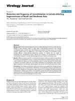
Figure 2a shows the variance functions of the QTL allelic effects in the
three scenarios. The polygenic and residual variances were the same for all
scenarios, and are shown in Figure 2b.
3.2. Analysis of the simu lated data
For each scenario 100 replicates were simulated as shown above. Repli-
cates were analysed using a random regression model with a cubic Legendre
polynomial for QTL, polygenic and residual effects. In each replicate two like-
lihood ratio tests were performed to test if the QTL was identified using the
random regression model and the traditional 305d model. Under both models,
the marker haplotypes were assumed known for grandsires, when the gametic-
relationship matrix was calculated. The restricted log-likelihoods were max-
imised using an Average Information REML procedure [8]. The maximisation
QTL analysis for function-valued traits 183
-0.6
-0.4
-0.2
0
0.2
0.4
0.6
a)
0 100 200 300
(
da
y
s
)
1.5
1.0

0.5
0.0
−0.5
−1.0
−1.5
Figure 1. Effect of the two alleles of the biallelic QTL in the three scenarios for the
simulated data. These effects are expressed as deviations from the fixed curve over
time (days).
184 M.S. Lund et al.
0
0.2
0.4
0.6
0.8
0 100 200 300 (days)
Scenario 1
Scenario 2
Scenario 3
a)
Figure 2. Variance function over time (days) in the three simulated scenarios due to
the QTL (a) and residual and polygenic effects (b). These figures are on the same scale
and can therefore be compared.
was performed every 3 cM over the simulated 100 cM interval. Data were anal-
ysed with a multiple allele model, although the simulated QTL was biallelic.
For the random regression model, the likelihood ratio test statistic was
LRT1 = L1/L2, where L1 and L2 are the maximum values of the re-
stricted log-likelihood under the models DYD = μ + Wq + Zu + e and
DYD = μ + Zu + e,whereq represents the QTL allelic effects, u the polygenic
effect, W and Z are the incidence matrices. The polygenic effect was simulated
according to a third order Legendre polynomial. It is therefore expected that

this effect will be perfectly fitted with this random regression model. The QTL
effect was simulated according to three different parametric functions of time,
as presented above.
In the 305d test, DYDmean for son s was calculated as the mean of his
55 DYD. The likelihood ratio test statistic was LRT2 = L3/L4, where L3 and
QTL analysis for function-valued traits 185
Table I. Statistical power of tests for the QTL detection in the simulation study in
the three different scenarios with a 305d model and a third order random regression
(i.e. number of times the simulated QTL was detected over 100 simulations).
Scenario 1 Scenario 2 Scenario 3
305d 62 16 6
Random regression 67 95 98
L4 are the maximum values of the restricted log-likelihood under the models
DYDmean = μ + Wq+ Zu + e and DYDmean = μ + Zu + e. Under the 305d
models the random polygenic and QTL allelic effects are multivariate normally
distributed such as: u ∼N(0,σ
2
a
A)andq|M, c ∼N(0,σ
2
q
Q|M, c), where M
corresponds to the marker data and c to the position on the chromosome. For
each of the 100 simulated replicates, the test statistic was compared to the
5% empirical threshold found by simulation over 500 replicates under the null
hypothesis.
3.3. Results on simulated data
The statistical power of the tests was calculated as the proportion of the
100 tests that were significant within each scenario and model type. As ex-
pected, when the QTL effect was constant over time the power of the two

models was comparable. On the contrary, in scenarios 2 and 3, where the
QTL effect was changing over time, the differences were substantial. In fact,
as shown in Table I, for the second scenario where the QTL allelic effects were
large during the first half of the period and nearly null during the second half,
the QTL was detected in 95 percent of the cases with the random regression
model and only 16 percent of the time with the 305d model. The difference
was even more pronounced for the third scenario where the average effect of
the two alleles was zero, although each allele had an important effect varying
during the whole time period. In this case, a considerable improvement was
achieved using a longitudinal model compared to a 305d analysis. Indeed, the
QTL was detected here in 98 percent of the cases with the random regression
model and only 6 percent of the time with the 305d model.
Given the estimated parameters of the random regression model, the vari-
ances can be calculated over time [9]. Figure 3 shows the average of the es-
timated curves of QTL variance over time over 100 replicates in the three
scenarios, as well as the curves based on simulation input parameters. Dif-
ferences observed for the first scenario are due to the fact that, in this case,
since the QTL effect was assumed to be constant over time, a constant term
186 M.S. Lund et al.
Figure 3. Curves of simulated (squares) and mean of estimated (triangles) variance
functions of QTL allelic effects over time in scenario 1 (a), scenario 2 (b), and sce-
nario3(c).
QTL analysis for function-valued traits 187
would have been more appropriate than a cubic polynomial. In fact, as al-
ready shown in previous studies [5], high order polynomials tend to become
extremely ‘wiggly’ and may not adequately fit simple covariance structures. In
practical cases, a likelihood ratio test can be performed to determine the most
appropriate order of the polynomial.
In the two other scenarios, however, when the QTL effect was assumed to
change with time, the variances were well estimated with the random regres-

sion model. Indeed, for the second simulated scenario, Figure 3b shows that
the random regression model was able to predict that the QTL effect was the
largest at the beginning of the time period. Similarly, Figure 3c shows that,
for the third scenario, the model adequately predicts a larger QTL effect at the
beginning and at the end of the time period. These estimations would be very
useful for genetic selection.
It has to be pointed out, however, that the proposed longitudinal model will
allow an increase of the detection power only if the QTL effect is sufficiently
large at least during some parts of the time period. A time-varying QTL with
asmalleffect during the whole lactation period will in fact not be detected.
On the contrary, if the time-varying QTL has a quite large overall effect it will
also be detected by the traditional 305d model. In this case, the improvement
reached with the longitudinal model will be the estimation of the QTL effect
over time, which will allow to know during which parts of the time period it
has the largest effect.
4. APPLICATION ON REAL DATA
In the dairy cattle breeding context, the use of test-day models to directly
analyse monthly (or even daily) milk production measurements is now used in
many different countries for genetic evaluation. It allows having more precise
genetic value estimations but also to select for the shape of the lactation curve
in order to improve, for instance, persistency. In these longitudinal models, the
polygenic effect of each individual is assumed to be changing with time, as
well as its variance and correlation functions. It is similarly expected in QTL
analyses that these specific genes will also have an effect changing over time.
Here, protein yield was used as an illustration of a longitudinal QTL detection
analysis.
4.1. QTL effect on protein yield in dairy cattle over the lactation
A granddaughter design was used with 19 grandsires and 1394 sons. Seven
chromosomes were scanned, which all had been previously reported in the
188 M.S. Lund et al.

literature to carry QTL for protein yield. For each chromosome, 4 to 12 mark-
ers were available. The exact names and positions of the markers for each
chromosome are available upon request from the first author.
All production data from the Danish HF database were used to calculate
DYD for each genotyped son. The model used for the DYD calculation is pre-
sented in detail by Lidauer et al. [10]. The only difference here is that the stage
of lactation was modelled with fixed regression terms, as in Lidauer et al. [10],
but nested within year*month of the test day. Two types of DYD for Danish
Holstein bulls were produced. The first were based on 305 day records and
produced one DYD per sire. The second were based on test day records and
produced time dependent DYD in 10 day intervals, resulting in about 30 mea-
surements along the lactation period (5 to 305 dim) for each sire.
Longitudinal QTL analyses were performed. Five different models were
compared for QTL detection. All five models include fixed, polygenic and
QTL effects. For the simple 305 day model, all the effects were assumed to be
constant. Four different random regression models were then considered. For
all of them, a third order Legendre polynomial was used for fixed and poly-
genic effects. Four different orders of Legendre polynomials were used for the
QTL effect over time: from a simple random intercept to a cubic Legendre
polynomial.
For each chromosome, the likelihood profile for the QTL detection was ob-
tained by maximising the likelihood every 3 cM. At the most likely position
on each chromosome a likelihood ratio test was performed. At present, a naive
chi-square test was used since the mixture of chi-square correction is not read-
ily applicable to compare the RR2 or RR3 model to the ‘no QTL’ model. The
degrees of freedom of the tests were calculated as the difference between the
number of parameters in the null model (with no QTL effect) and the longitu-
dinal model. The results presented here will therefore be slightly too conserva-
tive, but this should not alter the main aim of this study which was to compare
the 305 day model to various random regression models for QTL detection.

The QTL variance functions were estimated over the lactation to see at which
periods of time the QTL effect is likely to be the most important.
4.2. Results
Likelihood ratio test statistics for the seven scanned chromosomes for dif-
ferent orders of Legendre polynomials for the QTL effect are given in Ta-
ble II. The chromosomes were chosen based on QTL detection for protein
yield found in the literature. On this data set, however, the simple 305d model
QTL analysis for function-valued traits 189
Table II. Likelihood ratio test statistics of a 305 day model and random regression
models from a simple random intercept (RR0) to a third order Legendre polynomial
(RR3) for QTL effects. (Significant at 5% (*) and 1% (**) nominal levels from a
chi-square test. nc: not converged.)
BTA 305d RR0 RR1 RR2 RR3
9 0.9 0.0 0.6 9.3 12.4
10 1.1 0.1 8.6* 8.8 10.4
14 3.9* 7.9** 8.4* nc 7.2
20 0.2 1.1 9.8* 10.0 10.2
23 0.1 0.0 nc nc 5.2
26 2.5 3.4 5.4 11.9 13.6
27 0.0 1.1 9.8* nc 10.6
Figure 4. QTL variance functions over time at the maximum likelihood estimates
for the seven chromosomes for the protein yield data in dairy cattle. QTL explained
maximum 8% of the total genetic variance.
did not show enough power to detect any QTL for most of these chromosomes.
It was found, in this example, that the use of longitudinal models allowed to in-
crease the power of detection. This was especially observed on chromosomes
10, 20 and 27 for which QTL were not found significant with a 305 day model,
but were detected with a first order Legendre polynomial. The QTL variance
functions given in Figure 4 for these chromosomes show that the QTL on chro-
mosome 20 has a higher effect at the end of the lactation than at the beginning

and it is the contrary for the QTL detected on chromosome 27. For chromo-
some 10, the QTL has a quite large effect both at the beginning and the end of
the period while it is very small in the middle of the lactation.
190 M.S. Lund et al.
As shown in Figure 4, many QTL were found to have a large effect either at
the beginning or the end of the lactation period and very little over 305 days.
For the first group, they could be genes that contribute to high physiological
stress in the beginning of the lactation and might be most valuable as informa-
tion on QTL with pleiotropic effects on disease resistance. Such pleiotropy will
have to be verified in multiple trait analyses with functional traits. On the con-
trary, QTL with high effect at the end of the lactation will be more important
for persistency.
On chromosome 14, the QTL that was already detected with a 305 day
model was confirmed with the random regression model. Estimation of its vari-
ance over time (see Fig. 4), shows that its effect is large and nearly constant all
over the lactation period. It has to be emphasised, however, that the DGAT1
region was not covered here with markers which explains why the likelihood
ratio test statistics were not larger for this chromosome.
Table II shows that, for some QTL, the longitudinal effect was however quite
difficult to model and required a high order polynomial, and therefore a large
number of covariance parameters. This was especially the case for the QTL on
chromosome 9 that was best described by a third order Legendre polynomial.
Due to the large number of parameters involved, the likelihood ratio test for
the presence of a QTL was not found significant although the effect of this
QTL seems to be very large as shown in Figure 4. For this QTL, it might be
useful to try using more parsimonious longitudinal models, although the shape
of its variance and correlation functions might still be difficult to model with
few parameters.
This study showed that the use of random regression models increased the
power of detection of QTL that had a high effect for some parts of the lactation

but not the whole period. They also allow to see in which time periods the
effect of the QTL is the most important, which will be most useful for selection
to improve the shape of the lactation curve. The large number of parameters
involved in high order polynomials may, however, reduce the detection power
when the QTL effect is not large enough. This can be observed for example
in Table II for chromosome 14 with a third order Legendre polynomial. It is
therefore important to choose the most adequate polynomial order for each
QTL to avoid overfitting.
5. DISCUSSION
In QTL mapping studies, traits have often been defined as one record even
though it is a function of several measurements recorded over a time period.
QTL analysis for function-valued traits 191
An example is the 305 day milk yield, which is a weighted sum of a number of
measurements recorded over the lactation. Using the sum may be reasonable if
the genetic influence is constant over time. However, studies have shown that
correlations between measurements differ over the lactation [2, 24].
The results presented in this paper showed that the novel QTL-mapping
method, based on longitudinal models, provides an appropriate and powerful
tool to detect QTL affecting traits that are measured repeatedly over time. As
shown in the simulation study, the power to detect QTL increases substantially
compared to a standard 305d analysis, especially when the QTL-allelic effects
change over time. This is because, in the 305d model, the effect is averaged
over the whole period, and may thereby not be large enough to be detected. On
the contrary, the longitudinal models estimate the QTL variances and correla-
tions at all time points and uses the information of the QTL effect in each part
of the time period.
Analysis of the protein yield data in dairy cattle confirmed these results since
QTL with high effect at the beginning or the end of the lactation and very low
in the middle of the period were not detected with the simple 305 day model
but were found significant with the longitudinal approach. The use of these

models will therefore allow to detect new QTL that can have very important
impact on persistency, for instance, which is of particular interest to breeders.
Moreover, the methodology proposed here could be applied in marker assisted
selection and would bring much more precision in the genetic values as more
information is taken into account.
An issue still needs to be investigated, however, concerning the distribu-
tion of the likelihood ratio test statistics under the null hypothesis to detect
the presence of the QTL. In fact, in the real data analysis presented here a
naive chi-square distribution was assumed since the mixture of chi-square dis-
tributions are not known in the general case when a longitudinal QTL model
is used. Permutations are usually recommended to determine the significance
threshold but they can be in practice very computationally demanding and
time-consuming. More theoretical research is therefore required to find the
analytic distribution of the likelihood ratio test statistics for these longitudinal
QTL models.
As shown in the real data analysis, high order polynomials may be required
for the modelling of some QTL effects. In this case, the large number of param-
eters involved can prevent from detecting the QTL since the likelihood ratio
test may not appear significant. This problem might be overcome by the use
of more parsimonious longitudinal models such as character process [5, 20],
192 M.S. Lund et al.
or structured antedependence models [6]. This issue will be investigated in
further studies.
Our approach can easily be extended to multiple QTL detection as investi-
gated for single value characters by Lund et al. [12] as well as to the analysis of
multiple correlated function-valued traits such as milk production, protein and
fat contents. This QTL mapping approach can also be extended to the analysis
of binary or categorical traits, as proposed by Pletcher and Jaffrézic [21] in
polygenic models.
6. CONCLUSION

This study showed that the proposed model allowed to increase the power of
QTL detection when the QTL effect was overall too small to be detected with
classical methods but was still quite large during some part of the time period.
The proposed methodology also allows to have a more precise estimation of
the QTL effects over time. The longitudinal QTL approach therefore seems to
be a promising area of research for future studies in livestock populations.
ACKNOWLEDGEMENTS
We thank the Danish Cattle Federation for providing phenotypic data and
the Directorate for Food, Fisheries and Agri business for financial support.
REFERENCES
[1] Diggle P.J., Liang K.Y., Zeger S.L., Analysis of longitudinal data, Oxford
University Press, 1994.
[2] Druet T., Jaffrézic F., Boichard D., Ducrocq V., Modeling lactation curves and
estimation of genetic parameters for first lactation test-day records of French
Holstein cows, J. Dairy Sci. 86 (2003) 2480–2490.
[3] Fernando R.L., Grossman M., Marker-assisted selection using best linear unbi-
ased prediction, Genet. Sel. Evol. 21 (1989) 467–477.
[4] Grignola F.E., Hoeschele I., Tier B., Mapping quantitative trait loci in out-
cross populations via residual maximum likelihood, Genet. Sel. Evol. 28 (1996)
479–490.
[5] Jaffrézic F., Pletcher S.D., Statistical models for estimating the genetic ba-
sis of repeated measures and other function-valued traits, Genetics 156 (2000)
913–922.
[6] Jaffrézic F., Thompson R., Hill W.G., Structured antedependence models for ge-
netic analysis of multivariate repeated measures in quantitative traits, Genet. Res.
82 (2003) 55–65.
QTL analysis for function-valued traits 193
[7] Jakobsen J.H., Madsen P., Jensen J., Pedersen J., Christensen L.G., Sorensen
D.A., Genetic parameters for milk production and persistency for Danish
Holsteins estimated in random regression models using REML, J. Dairy Sci.

85 (2002) 1607–1616.
[8] Jensen J., Mantysaari E., Madsen P., Thompson R., Residual maximum likeli-
hood estimation of (co)variance components in multivariate mixed linear models
using average information, J. Indian Soc. Agric. Stat. 49 (1997) 215–236.
[9] Kirkpatrick M., Heckman N., A quantitative genetic model for growth, shape, re-
action norms, and other infinite-dimensional characters, J. Math. Biol. 27 (1989)
429–450.
[10] Lidauer M., Pedersen J., Pösö J., Mäntysaari E.A., Strandén I., Madsen P., Nielen
U.S., Eriksson J A., Johansson K., Aamand G.P., Joint Nordic Test Day Model:
Evaluation Model, Interbull Bull. 35 (2006) 103–107.
[11] Lund M.S., Sorensen P., Madsen P., Linkage analysis in longitudinal data using
random regression, Proc. 7th WCGALP, 32, 713-716, CD-rom Communication
No 21-28, Montpellier, France, 2002.
[12] Lund M.S., Sorensen P., Guldbrandsten B., Sorensen D.A., Multitrait fine map-
ping of quantitative trait loci using combined linkage disequilibria and linkage
analysis, Genetics 163 (2003) 405–410.
[13] Ma C.X., Casella G., Wu R., Functional mapping of quantitative trait loci un-
derlying the character process: a theoretical framework, Genetics 161 (2002)
1751–1762.
[14] Macgregor S., Knott S.A., White I., Visscher P.M., Longitudinal variance-
components analysis of the Framingham heart study data, BMC Genetics 4
(2003) S22, 5 p.
[15] Macgregor S., Knott S.A., White I., Visscher P.M., Quantitative trait locus anal-
ysis of longitudinal quantitative trait data in complex pedigrees, Genetics 171
(2005) 1365–1376.
[16] Madsen P., Sørensen P., Su G., Damgaard L.H., Thomsen H., Labouria R.,
DMU - a package for analyzing multivariate mixed models, Proc. 8th WCGALP,
CD-rom Communication No 27-11, Belo Horizonte, Brazil, 2006.
[17] Meuwissen T.H.E., Goddard M.E., Fine mapping of quantitative traits using link-
age disequilibria with closely linked marker loci, Genetics 155 (2000) 421–430.

[18] Meyer K., Grasser H.U., Hammond K., Estimates of genetic parameters for first
lactation test day production of Australian black and white cows, Livest. Prod.
Sci. 21 (1989) 177–199.
[19] Moreno C.R., Elsen J.M., Le Roy P., Ducrocq V., Interval mapping methods for
detecting QTL affecting survival and time-to-event phenotypes, Genet. Res. 85
(2005) 139–149.
[20] Pletcher S.D., Geyer C.J., The genetic analysis of age-dependent traits: modeling
a character process, Genetics 153 (1999) 825–833.
[21] Pletcher S.D., Jaffrézic F., Generalized character process models: estimating the
genetic basis of traits that cannot be observed and that change with age or envi-
ronmental conditions, Biometrics 58 (2002) 157–162.
194 M.S. Lund et al.
[22] Rodriguez-Zas S.L., Southey B.R., Heyen D.W., Lewin H.A., Detection of quan-
titative trait loci influencing dairy traits using a model for longitudinal data, J.
Dairy Sci. 85 (2002) 2681–2691.
[23] Wang T., Fernando R.H., van der Beek S., van Arendonk J.A.M., Covariance be-
tween relatives for a marked quantitative trait locus, Genet. Sel. Evol. 27 (1995)
251–274.
[24] White I.M.S., Thompson R., Brotherstone S., Genetic and environmental
smoothing of lactation curves with cubic splines, J. Dairy. Sci. 82 (1999)
632–638.
[25] Wu R., Hou W., A hyperspace model to decipher the genetic architecture
of developmental processes: allometry meets ontogeny, Genetics 172 (2006)
627–637.