Báo cáo sinh học: "A comparison between Poisson and zero-inflated Poisson regression models with an application to number of black spots in Corriedale sheep" doc
Bạn đang xem bản rút gọn của tài liệu. Xem và tải ngay bản đầy đủ của tài liệu tại đây (314.79 KB, 16 trang )
Original article
A comparison between Poisson
and zero-inflated Poisson regression models
with an application to number of black spots
in Corriedale sheep
Hugo NAYA
1,2,3
*
, Jorge I. URIOSTE
2
, Yu-Mei CHANG
3
,
Mariana R
ODRIGUES-MOTTA
3
, Roberto KREMER
4
, Daniel GIANOLA
3
1
Unidad de Bioinforma´tica, Institut Pasteur de Montevideo, Mataojo 2020,
Montevideo 11400, Uruguay
2
Departamento de Produccio´n Animal y Pasturas, Facultad de Agronomı´a, Av. Garzo´n 780,
Montevideo 12900, Uruguay
3
Department of Animal Sciences, University of Wisconsin-Madison, Madison,
WI 53706, USA
4
Departamento de Ovinos y Lanas, Facultad de Veterinaria, Av. Lasplaces 1550,
Montevideo 11600, Uruguay
(Received 15 October 2007; accepted 16 January 2008)
Abstract – Dark spots in the fleece area are often associated with dark fibres in wool,
which limits its competitiveness with other textile fibres. Field data from a sheep
experiment in Uruguay revealed an excess number of zeros for dark spots. We compared
the performance of four Poisson and zero-inflated Poisson (ZIP) models under four
simulation scenarios. All models performed reasonably well under the same scenario for
which the data were simulated. The deviance information criterion favoured a Poisson
model with residual, while the ZIP model with a residual gave estimates closer to their
true values under all simulation scenarios. Both Poisson and ZIP models with an error
term at the regression level performed better than their counterparts without such an
error. Field data from Corriedale sheep were analysed with Poisson and ZIP models with
residuals. Parameter estimates were similar for both models. Although the posterior
distribution of the sire variance was skewed due to a small number of rams in the dataset,
the median of this variance suggested a scope for genetic selection. The main
environmental factor was the age of the sheep at shearing. In summary, age related
processes seem to drive the number of dark spots in this breed of sheep.
zero-inflated Poisson / sheep / spot / posterior predictive ability / Bayesian hierarchical
model
*
Corresponding author:
Genet. Sel. Evol. 40 (2008) 379–394
Ó INRA, EDP Sciences, 2008
DOI: 10.1051/gse:2008010
Available online at:
www.gse-journal.org
Article published by EDP Sciences
1. INTRODUCTION
The presence of black-brown fibres in wool from Corriedale sheep is recogni-
sed as a fault [13,20]. This issue limits the competitiveness of wool with other
textile fibres and reduces its value by 15–18% wh en the number exceeds
300 fibresÆkg
À1
top (Frank R acket, 1997, personal communication). In Ur uguayan
wool, this value can be as large as 5000 fibresÆkg
À1
top, wi th most of the dark
fibres having an environmental origin, e.g. faeces and urine dyeing [3,18]. W ith
appropriate clip preparation, values ranging from 800 to 1000 fibres have been
found, and these probably have a genetic background. Skin spots with black-
brown fibres and isolated pigmented fibres are the probable origin of these fibres
[2,9,12,20].
W ith the aim of investigating factors involved i n the development of pig-
mented fibres, an experiment was carried out in which fleeces of animals from
two experimental flocks were sampled yearly at she aring for laboratory analysis.
Each animal was inspected, and the number of black spots, their diameter and
the estimated percentage of dark fibres in each spot were recorded. W hile
genetic selection should focus on reducing the number of dark fibres, it is expen-
sive and cumbersome to record such a value for each animal on a routine basis.
Laboratory techniques are labour intensive and slow.
In this context, the number of dark spots i n the fleece area of animals may be
a useful indicator trait, for several reasons. First, our empirical observations sug-
gest that dark fibres are associat ed with dark spots , hinting a positive correlation
between the two variables. Second, spots can be assessed easily and quickly, and
scoring is less subjective than for other candidate measures such as the percent-
age o f spot area with dark fibres [1,10,11]. Third, we have observed that in spots
without or with dark fibres in young animals, the presence of d a rk fibres
increases with age. Hence, the presence of spots indicates dark fibres in adult
animals. If laboratory analyses confirm that black spots are positively correlated
with the number of dark fibres, recording on a nation-wide basis wo uld be
straightforward.
Previous studies in Romney sheep [6] ha ve addressed the occurrence of black
wool spots at weaning (BWS
w
) and at yearling age (BWS
y
). Enns and Nicoll [6]
used a threshold model for a binary response variable (the presence or absence
of pigmented spots), and their largest heritability estimates were 0.070 (0.018)
and 0.072 (0.014) for BWS
w
and BWS
y
, respectively. In contrast, in our
research, focus has been on modelling the number of dark spots in each animal,
irrespective of the presence of dark fibres. As a count variable, the number of
spots coul d plausibly follow a Poisson distribu tion. However , as show n in
Figure 1, there is an excess of zeros in the empirical distribution for field records,
380
H. Naya et al.
relative to their expected value under Poisson sampling with a homogeneous
parameter. If Y follows a Poisson distribution, then E(Y)=Var(Y), where E(Æ)
and Var(Æ) repr esent the mean and variance, respectively. In a Poisson distribu-
tion, the variance-to-mean-ratio (VTMR) is 1. In the observed data in Figure 1,
VTMR was 6.8. A zero-inflated Poisson model (ZIP) [17], may provide a better
description of the data. This model assumes that observations come from one of
two dif ferent components, a ‘‘perfect’’ state which produces only zeros with
probability h, and an ‘‘imperfect’’ one that follows a Poisson distribution, with
probability (1 À h) and Poisson parameter k. It can be shown that the mean and
variance of a ZIP variate are
EðY Þ¼ð1 À hÞk ð1Þ
and
VarðY Þ¼EðY Þð1 þ hkÞ; ð2Þ
respectively, which accounts for VTMR > 1 provided that overdispersion
arises from an excess of zeros. Zero-inflated models for count data in animal
breeding have been discussed by Gianola [15] and used by Rodrigues-Motta
and collaborators [27] in an analysis of the number of mastitis cases in dairy
cattle.
Figure 1. Distribution of the number of black spots in field data (n = 497). The solid
line represents the best fit of a Poisson distribution to the observed data, fitted with
package ‘‘gnlm’’ ( [ 26 ].
Poisson and ZIP models for spots in sheep
381
From previous exploratory analysis [16,24], the age of animals appears to be
a main source of variability of the number of spots, with flock and year having
marginal effects. Modelling can proceed along the lines of generalised linear
models [21] or generalised linear mixed m odels [25] provided that the link func-
tion used is appropriate. However when mixture distributions are assumed, as in
the ZIP model, estimation is more involved, since indicator variables (e.g.,from
which of the two states a zero originates) are not observed. However, imputation
of non-observed parameters given the data fits naturally in the Bayesian frame-
work [19]. In recent years, Bayesian Markov chain Monte Carlo (MCMC) meth-
ods have become widely used in animal breeding [28], as a powerful and
flexible tool. An advantage of the Bayesian MCMC framework is that it is rel-
atively easy to implement measures of model quality such as posterior predictive
ability (PPA) checks.
In this paper, four different candidate models for the number of spots w ere
compared. Poisson and ZIP models were considered, with the log of the Poisson
parameter of each of the models regressed on environmental and genetic effects.
The two models were extended further to include a random residual in the
regression, aimed to capture overdispersion other than that due to extra zeros.
Two of the models were selected and fitted to a sample of Corriedale sheep
to obtain estimates of population parameters.
2. MATERIALS AND METHODS
2.1. Simulation
Four diff erent scenarios (H1–H4) were simulated as described in Table I.The
rationale und erlying the models is that the observed number of s pots in each ani-
mal follows a Poisson distribution wi th the logarithm of its parameter expressed as
a linear model. The Poisson distribution does not accommodate well the overdis-
persion caused by excess zeros, so a ZIP m odel is a reasonable competitor. Further-
more, the parameter of the Poisson distribution represents the expected propensity
of spots, so an additional error (residual) term at the regression level a llows mod-
elling individual differences in propensity. The two models (Poisson and ZIP),
each with or without residuals, give the four models (P, Z, Pe and Ze) studied.
Data were generated from either ZIP (H1, H2) or Poisson (H3, H4) distribu-
tions; the log of the Poisson parameter contained (H2, H4) or did not contain
(H1, H3) a random residual. In all four models, the ram effects were assumed
to follow independent normal distributions with null mean and variance r
2
ram
;
the residual was independent and identically distributed as e
i;j;k
$ Nð0; r
2
e
Þ
(H2, H4).
382
H. Naya et al.
In each scenario, 100 datasets (replicates) were randomly generated, with
1000 observations each. For each animal, the covariate age was randomly sam-
pled, resembling the distribution of the age in the observed data. Forty rams
(sires) were sampled in each dataset and randomly assigned to observations.
In e ach scenario, the true parameters were selected to resemble the observed dis-
tribution of spots.
2.2. Models fitted in the simulation
Four models were fitted to the simulated data (Z, Ze, P and Pe), each match-
ing a specific scenario, as shown in Table I. Models are connected as illustrated
in Figure 2. A path between two models involves fixing or adding a single
parameter. Preliminary analysis indicated that flock and year effects (and their
interaction) had minor importance, so these factors were not included in the sim-
ulations. However, when m odels were fitted to the real data, the regression mod-
els included flock and year effects.
2.3. Bayesian computation
Parameter inference was done using the Op enBUGS software [31]. Va gue
priors were assigned to represent initial uncertainty. A normal distribution centred
at zero with precision 0.01 was used for location parameters, wh ile a Gamma
(0.01, 0.01) distribution was assumed for each of the two variance parameters.
Several different hyper -parameter values were assigned in pilot runs, with the
only observable difference being the time needed to attain convergence. For each
scenario and model, the burn-in period was determined from preliminary runs,
based on four chains, starting at different points. Final runs were performed
with two chains each. The burn-in period was of 10 000 iterations, and samples
were obtained from the following 10 000 iterations, without thinning. An
exception was model Pe in scenario H4, where the required burn-in period
was 30 000 iterations.
Table I. Model label, simulated data distribution given the parameters, regression
function and name of each scenario (H1, H2, H3, H4).
Model Distribution Regression Scenario
Z y
i;j;k
$ ZIPðh; k
i;j
Þ logðk
i;j
Þ¼b
0
þ b
1
Á age
i
þ ram
j
H1
Ze y
i;j;k
$ ZIPðh; k
i;j;k
Þ logðk
i;j;k
Þ¼b
0
þ b
1
Á age
i
þ ram
j
þ e
i;j;k
H2
P y
i;j;k
$ Poissonðk
i;j
Þ logðk
i;j
Þ¼b
0
þ b
1
Á age
i
þ ram
j
H3
Pe y
i;j;k
$ Poissonðk
i;j;k
Þ logðk
i;j;k
Þ¼b
0
þ b
1
Á age
i
þ ram
j
þ e
i;j;k
H4
The b’s are unknown regressions.
Poisson and ZIP models for spots in sheep
383
2.4. End points for model comparison
Models were contrasted first through simulated data (comparing true and esti-
mated parameter values) and by using the deviance information criterion (DIC),
estimates of marginal likelihoods with the method of Newton and Raftery [22]
and via PPA. The DIC [30] was obtained directly from OpenBUGS.PPAwas
patterned after Sorensen and Waagepetersen [29 ]. Suppose that for a model
M, h
ðkÞ
M
, k =1, , K, is drawn from the posterior distribution of the parameter
vector h
M
, and that, subsequently, replicate data y
ðkÞ
M
are generated given h
ðkÞ
M
as
true parameters. Given some univariate discrepancy statistic T ðy; h
M
Þ, it is pos-
sible to study the predictive ability of model M from samples drawn from the
posterior distribution of the difference T ðy; h
ðkÞ
M
ÞÀT ðy
ðkÞ
rep
; h
ðkÞ
M
Þ. For the Poisson
model we used
T y; h
M
ðÞ¼
X
K
k¼1
y À k
k
ffiffiffiffiffi
k
k
p
2
ð3Þ
Figure 2. Graphical display of the four models considered. Distances depend on one
or two parameters. h is probability of the perfect state; r is the standard deviation of
the error term in the regression. Dashed line s connect models that need to incorporate
one parameter while fixing the other parameter to zero.
384 H. Naya et al.
as discrepancy statistic, where k
k
in the numerator is the mean, and
ffiffiffiffiffi
k
k
p
in the
denominator is the standard deviation; for the ZIP model, the mean and stan-
dard deviation were replaced by their corresponding values.
2.5. Field data
Records were collected in 2002–2004 from two experimental flocks belong-
ingtotheUniversidaddelaRepu´ blica, Uruguay. After edits, 497 records from
sheep with known sire (ram) were kept; 37, 182 and 278 records were from
2002, 2003 and 2004, respectively; 407 and 90 were from flocks 1 and 2,
respectively. Genetic connection was through two rams with progeny in both
flocks; a t otal of 19 rams had progeny. In our dataset 36 animals had records
in both 2002–2003, 71 in 2003–2004 and 27 animals had measures in all three
years. For simplicity, dependence between observations from the same a nimal
was ignored, so that the only source of correlation considered was that resulting
from a half-sib family structure. Clearly, the limited dataset precludes precise
estimation of genetic parameters, but this was not an objective of this study.
3. RESULTS
3.1. Simulations
For each scenario simulated, the results are presented for the ‘‘true’’ model
and for the other three models. Values of the DIC (highlighting pD, the ‘‘effec-
tive number of parameters’’) and of the difference statistic used for PPA are
showninTableII.
3.1.1. DIC
In scenario H1, where Z is the true model, Pe performed better (lower DIC)
than the true model, in spite of the penalty resulting from a larger pD (number of
parameters). The value of nearly 400 effective parameters in 1000 observations
indicates that very few observations clustered under the same Poisson di stribu-
tion. Models with residuals had a higher pD but lower deviance. Except for the
P model, the other specifications had similar DIC, at least in the light of the
between replicates standard deviation. Clearly the Poisson model was the worst
under the ‘‘true ZIP’’ scenario.
In scenario H2 (Ze is the true model), Pe was, again, better than the true
model and the picture with respect to pD was as in the H1 scenario, although
differences between models with residuals were smaller . Models without resid-
uals had the poorest performance; P had the worse DIC.
Poisson and ZIP models for spots in sheep
385
Under H3 (P is the true model) all DIC values were similar. Models with
residuals had smaller pD than in scenarios H1, H2, probably due to the simpler
nature of this simulation scenario. Finally, in scenario H4, the true model (Pe)
was best under the DIC, followed by Ze.
The global picture is clearer when the number of times (in 100 simulations) in
which each model had the smallest DIC was considered (Tab. III). Model Pe
outperformed other models except under H3. No tably, DIC selected the right
model only in 172 out of 400 comparisons (43% of the time).
Table III. Times a given model was the best when selected by DIC (over
100 replicates).
Fractional numbers correspond to ties. The ‘‘true’’ models are in the diagonal while the
‘‘winner’’ model for each scenario is shown in boldface.
Model ZZe P Pe
H1 0.5 0.5 0.0 99
H2 0 0 0 100
H3 2 3.5 77.5 17
H4 1 0 0 99
Table II. Averages and standard deviations of deviance information criterion (DIC),
effective number of parameters (pD) and difference statistic for the posterior
predictive ability (DPPA) for the four model s in each scenario over 100 replicates.
Scenario Model DIC s.d. pD s.d. DPPA s.d.
H1 Z 2368.0 101.8 17.3 1.3 0.003 0.030
Ze 2368.9 101.5 34.1 6.8 À0.006 0.028
P 3138.5 196.6 17.8 0.8 1.204 0.137
Pe 2262.5 102.7 399.6 18.9 0.050 0.009
H2 Z 2645.1 117.4 18.1 1.0 0.175 0.055
Ze 2521.3 103.7 135.0 17.8 0.00 7 0.011
P 3579.9 222.3 18.2 0.6 1.878 0.239
Pe 2308.2 101.7 431.3 18.1 0.030 0.009
H3 Z 1768.4 77.8 16.8 1.1 À0.006 0.049
Ze 1769.9 77.5 31.9 6.3 À0.021 0.050
P 1766.6 77.9 16.7 1.0 0.007 0.052
Pe 1768.2 77.8 33.1 6.3 À0.007 0.046
H4 Z 1962.9 127.7 17.8 1.0 0.177 0.085
Ze 1848.2 84.3 125.1 20.1 À0.006 0.033
P 1958.4 107.5 17.3 1.0 0.276 0.101
Pe 1842.7 84.1 131.8 19.0 0.00 7 0.034
The model corresponding to each scenario is in boldface.
386 H. Naya et al.
3.1.2. PPA
Values of the PPA difference statistic c lose to zero indicate essentially no dif-
ferences betwe en observed and predicted responses. In regard to the PPA results,
the true model always predicted best, and this was essentially true for all scenar-
ios (Tab. II). The pure Poisson model (P) performed badly in ZIP scenarios (H1
and H2), wh i le Ze did reasonably well in all four scenarios. In H3, PPA wa s sim-
ilar for all models. The problem with this criterion seems to be its low discrim-
inative power , relative to its high standard deviations over replications.
Alternatives to PPA are cross-validation techniques, but these were not consid-
ered due to computational expense.
3.1.3. Marginal likelihood
It was impossible to calculate the Bayes factor for several pairs of models,
given the huge differences in marginal likelihoods. For this reason, only esti-
mates of marginal log-likelihood are presented for each model and scenario
(Tab. IV). On the basis of this criterion, Pe was the best model in all scenarios.
3.1.4. Parameter inference
As expected, parameter estimates were in agreement with their ‘‘true’’ values
when a model matched its corresponding scenario (Tab. V). Ho wever, when
models pertained to a different scenario, their performances were markedly dif-
ferent. Regressions on age were well inferred, but estimated intercepts b
0
were
severely understated when Poisson models were applied to ZIP scenarios. Model
Ze estimates were always in agreement with the ‘‘true’’ values, regardless of the
scenario. Pe model estimates of intercept and of the residual variance were
strongly biased in ZIP scenarios. Finally, models with residuals estimated the
sire (ram) variance well.
The ability of different models to pre dict breeding values is of interest. Gi ven
that the ‘‘true’’ values of rams were known, their Spearman rank correlation with
Table IV. Mean and standard deviation (in 100 runs) of the harmonic mean of sampled
log-likelihoods for each model and scenario.
Model Z s.d. Ze s.d. P s.d. Pe s.d.
H1 À1184.1 50.5 À1180.2 50.6 À1569.1 98.3 À1007.7 44.8
H2 À1322.4 58.5 À1235.7 51.0 À1789.6 111.0 À1012.5 46.0
H3 À884.8 38.6 À881.4 38.5 À883.9 38.8 À880.2 38.8
H4 À974.5 53.0 À902.8 40.0 À979.4 53.7 À898.9 40.3
Poisson and ZIP models for spots in sheep
387
the predicted va lues (posterior mean) was calculated for each combination of
scenarios and models. Ze was best in all scenarios, but differences were small
(Fig. 3). The ZI P model performed reasonably well in all scenarios, while pure
Poisson models did well only in their own scenarios, with median correlations
between 0.41 and 0.53.
Figure 3. Histograms of Spearman rank correlations between true and posterior
means of ram breeding values. H4 scenario for models Pe (a) and Ze (b).
388 H. Naya et al.
3.2. Field data
Given the simulation results, data were analysed using the two ‘‘best’’ mod-
els, Pe and Ze, including flock, year, flock · year and age effect as covariates,
and ram as a genetic effect. The effects were removed successively from each
main model and DIC was computed; full models were found to be the best.
Since the effects of flock, year and flock-year interaction were negligible, these
arenotreportedinTableVI.DIC(pD) was 1 103 (200.6) and 1070 (201.8) for
the Ze and Pe models, respectively. The number of spots increased with age, and
there was no strong evidence of inflation at zero (the estimate of the probability
of the perfect state, h, was 0.05). It seems that most of the overdispersion is due
to unaccounted for between-individual variability.
Table V. Parameter estimates for the four scenarios by model.
Model b
0
s.d. b
age
s.d. r
2
ram
s.d. r
2
e
s.d. h s.d.
H1 À0.500 0.520 0.090 0.000 0.510
Z À0.503 0.097 0.521 0.017 0.104 0.042 0.504 0.022
Ze À0.525 0.102 0.523 0.018 0.102 0.042 0.022 0.010 0.500 0.023
P À1.236 0.123 0.524 0.038 0.169 0.072
Pe À1.869 0.142 0.493 0.044 0.103 0.057 1.666 0.177
H2 À0.550 0.520 0.090 0.250 0.480
Z À0.282 0.133 0.492 0.032 0.130 0.051 0.524 0.025
Ze À0.526 0.139 0.515 0.028 0.101 0.046 0.251 0.058 0.482 0.028
P À1.089 0.148 0.511 0.043 0.186 0.064
Pe À1.840 0.151 0.471 0.051 0.094 0.052 2.029 0.214
H3 À2.500 0.850 0.090 0.000 0.000
Z À2.477 0.102 0.845 0.017 0.102 0.041 0.014 0.006
Ze À2.485 0.108 0.845 0.017 0.099 0.040 0.018 0.009 0.014 0.005
P À2.497 0.104 0.848 0.017 0.102 0.039
Pe À2.511 0.107 0.849 0.016 0.100 0.038 0.019 0.009
H4 À2.500 0.810 0.090 0.250 0.000
Z À2.268 0.347 0.793 0.053 0.140 0.052 0.063 0.087
Ze À2.470 0.122 0.810 0.025 0.104 0.046 0.221 0.056 0.022 0.010
P À2.397 0.137 0.810 0.030 0.143 0.053
Pe À2.509 0.122 0.814 0.025 0.105 0.046 0.237 0.055
The ‘‘true’’ value of each parameter is given in the line corresponding to each scenario (H1–
H4). Estimates for which the ‘‘true value’’ is inside a 2 standard deviations region are in
boldface (see text for definition of parameters).
Poisson and ZIP models for spots in sheep
389
In standard animal breeding theory, in a sire model, heritability is defined as:
h
2
¼
4r
2
ram
r
2
ram
þ r
2
e
Áð4Þ
Estimates of heritability (in a log-scale) under the two models considered are
displayed in Table VI. Posterior medians were 0.25 and 0.17 for the Ze and Pe
model, respectively, but the distribution was very skewed due to the few rams
(19) used in the study.
4. DISCUSSION
While easier to measure than the number of dark fibres per animal, modelling
the number of spots poses several challenges in regard to standard methodology
of animal breeding. It is very difficult to obtain a good fit of the data with simple
linear models with normal distributions for the random effects. Frequently used
Box-Cox transformations (e.g., log or reciprocal) cannot be us ed, given the num-
ber of zeros. Additionally, there is the issue of an excess of zeros relative to
Poisson sampling. One at tractive model for dealing with this is the ZIP. One
can think of a fraction h of ‘‘perfect’’ animals that will never develop spots,
whereas others only will develop spots at random, following a Poisson
distribution with parameter k. Moreover, va riation in the k’s can be accounted
for by a model including environmental and genetic factors, such as age, flock,
year or ram.
We first compared the performance of four models (i.e., Poisson and ZIP with
and wi thout an error term in the regression) using a simulation that resembled
the field data structure. Based on the end points considered, two ‘‘competitive’’
Table VI. Posterior median and quantiles (2.5% and 97.5%) of the distribution of
parameters, and difference in posterior predictive ability (DPPA) for Pe and Ze
models applied to field data.
Model Ze Pe
2.5% Median 97.5% 2.5% Median 97.5%
b
0
À2.490 À1.692 À0.926 À2.622 À1.884 À1.185
b
age
0.465 0.611 0.761 0.485 0.628 0.772
r
2
ram
0.008 0.092 0.474 0.008 0.086 0.460
r
2
e
1.308 1.854 2.567 1.513 2.026 2.736
h 0.002 0.050 0.173
Heritability 0.023 0.246 0.836 0.016 0.166 0.714
DPPA À0.471 À0.038 0.406 À0.500 À0.040 0.423
390 H. Naya et al.
models emerged, Pe and Ze, both including residuals. Fitting hierarchical mod-
els with an error term such as Pe and Ze can be viewed as a log-normal mixture
of Poisson and ZIP distributions, respectively [5]. This provides a very flexible
structure, which explains at least partially, the good performance of these two
models in the simulation results.
Using the DIC, the Pe model was best in most scenarios, in spite of a larger
pD, a term that penalises the likelihood and that is associated with the effective
number of parameters of the model. The results of the marginal likelihoods also
supported this interpretation (Tab. IV), while the difference statistic for the pos-
terior predictive ability (DPPA) displayed low discriminative power. However,
the Pe model did not produce good estimates of the intercept (number of spots
at age = 0, i.e. birth) and of the residual variance, when data were generated from
ZIP distributions (Tab. V). This suggests that even the results of DIC should be
viewed with some caution. Furthermore, as pointed out by several discussants in
Spiegelhalter et al.[30], the DIC may underpenalise model complexity. Several
alternative versions of DIC were proposed by Celeux et al.[4] to address models
with missing data or mixtures of distributions. Ho wever, despite important differ-
ences in performance, each alternative proposed has its own drawbacks and no
single solution emerges as unanimously appropriate.
On the contrary, Ze wa s robust across all situations, since it estimated the true
parameters well. A ‘‘stable model’’ is appealing under practical conditions. In
animal breeding, a s table model with good predictive ability is desired. All mod-
els produced a good agreement between ‘‘ true’’ and predicted breeding values,
especially Ze, which maintained its ability across scenarios.
Based on the simulation, Pe and Ze were chosen to analyse the field dataset.
As expected, under the DIC Pe outperformed Ze. However, parameter estimates
were similar (Tab. VI). This may be explained by the fact that the estimate of h
in Ze was low, pointing to a relatively small effect of ‘‘perfect’’ individuals on
inference when the Poisson model includes a residual.
A series of environmental and genetic f actors may be related to the number of
spots. Simple observation (even in humans) suggests that this number increases
with age and environmental stress factors (e.g., solar irradiation can be invo ked
as causative agents [7,8,14,23]). Variability in the underlying genetic
mechanisms responsible for the spots is likely, at least in different races, as well
as in susceptibility to environmental stress factors.
The age of the animals was the main environmental factor to consider, con-
sistently. However, it is not known if this relationship arises from an intrinsic
ageing process independent of environmental factors, or if environmental stress-
ors such as sun irradiation drive the process. Anyhow, it is possible to envisage
management measures aiming to reduce incidence of dark fibres. If an intrinsic
Poisson and ZIP models for spots in sheep
391
ageing process is the main factor , reducing the age at shearing could be a prac-
tice to take into consideration. This requires additional research.
In an animal breeding context, genetic and environmental variances are extre-
mely important since they define herit ability, a key parameter used to select
among breeding strategies. The meaning of h eritability in non-linear hierarchical
models, such as Pe or Ze, is not straightforward. However , the magnitude of her-
itability suggests scope for genetic selection. Different simulations indicated that
predicted breeding values (for log k) were in good agreement with ‘‘true’’ val-
ues, so these models are probably useful for selection purposes.
In summary, hierarchical models for count data were studied with the aim of
defining strategies for reducing incidence of dark fibres in wool from Corriedale
sheep. ZIP and Poisson models with random residuals performed better than
their counterparts without residuals. Ageing related processes seem to drive
the number of dark spots in sheep, and further research should be done to
address this underlying phenomenon.
ACKNOWLEDGEMENTS
We would like to thank the Associate Ed itor and two anonymous reviewers
for their useful comments and suggestions, and Gonzalo I. Pereira, Carlos R.
Lopez, Lucı´a Surraco and Fabia´n Gonzalez for field data collection. We are
indebted to Gustavo de los Campos, Guilherme J.M. Rosa, Agustı´ n Blasco
and Martı´n Gran˜a for helpful discussions. This work was partially supported
by Comisio´n Sectorial de Investigacio´n Cientı´fica – Uruguay, and by grant
PDT35-02 from Programa de Desarrollo Tecnolo´gico (Ur uguay). Support from
the Wisconsin Ag riculture Ex periment Station, and from grant NSF DMS-NSF
DMS-044371 is also acknowledged.
REFERENCES
[1] Cardellino R., Herencia de fibras coloreadas, Produc. Ovina 6 (1994) 19–37.
[2] Cardellino R., Mendoza J., Fibras colore adas en tops con lanas acondicionadas
(zafra 94–95), Rev. Lananoticias SUL 115 (1996) 37–40.
[3] Cardellino R., Guillamo´n B.E., Severi J.F., Origen de las fibras coloreadas en tops
de lana uruguaya, Produc. Ovina 3 (1990) 81–83.
[4] Celeux G., Forbes F., Robert C.P., Titterington D.M., Deviance information crite-
ria for missing data models, Bayesian Anal. 1 (2006) 651–674.
[5] Draper D., Tutorial 1: Hierarchical Bayesian Modeling, in: 6th World Meeting
International Society for Bayesian Analysis, 28 May–1 June, 2000, Hersonissos,
Heraklion, Cr ete.
392 H. Naya et al.
[6] Enns R.M., Nicoll G.B., Incidence and heritability of black wool spots in
Romney sheep, N. Z. J. Agric. Res . 45 (2002) 67–70.
[7] Fears T.R., Scotto J., Schneiderman M.A., Skin cancer, melanoma, and sunlight,
Am. J. Public Health 66 (1976) 461–464.
[8] Fears T.R., Scotto J., Schneiderman M.A., Mathematical models of age and ultra-
violet effects on the incidence of skin cancer among whites in the United States,
Am. J. Epidemiol. 105 (1977) 420–427.
[9] Fleet M., Pigmentation types. Understanding the heritability and importance,
Wool Tech. Sheep Breed. 44 (1996) 264–280.
[10] Fleet M.R., Forrest J.W., The occurrence of pigmented skin and pigmented wool
fibres in adult Merino sheep, Wool Tech. Sheep Breed. 33 (1984) 83–90.
[11] Fleet M., Lush B., Sire effects on visible pigmentation in a Corriedale flock,
Wool Tech. Sheep Breed. 45 (1997) 167–173.
[12] Fleet M.R., Ponzoni R.W., Fibras pigmentadas en vellones blancos, in: Larrosa
J.R., Bonifacino L.A. (Eds.), Seminario Cientı´fico Te´cnico Regional de Lanas,
Montevideo, 1985, pp. 135–142.
[13] Fleet M.R., Stafford J.E., The association between non-fleece pigmentation and
fleece pigmentation in Corriedale sheep, Anim. Prod. 49 (1989) 241–247.
[14] Forrest J.W., Fleet M.R., Pigmented spots in the wool-bearing skin induced by
ultraviolet light, Aust. J. Biol. Sci. 39 (1986) 123–136.
[15] Gianola D., Statistics in animal breeding: angels and demons, in: Proceedings of
the 8th World Congress on Gene tics Applied to Livestock Production, 13–18
August, 2006, CD Paper 00-03, Belo Horizonte-MG, Brazil, 8 p.
[16] Kremer R., Urioste J.I., Naya H., Rose´s L., Rista L., Lo´pez C., Incidence of skin
spots and pigmentation in Corriedale sheep, in: IX World Conference on Animal
Production, 26–31 October, 2003, Porto Alegre, Brazil.
[17] Lambert D., Zero-inflated Poisson regression, with an application to defects in
manufacturing, Technometrics 34 (1992) 1–14.
[18] Larrosa J.R., Orlando D., Incidencia de fibras oscuras en lanas peinadas
uruguayas, in: An. Fac. Vet. Uruguay, Montevideo, 21/25, 1984–1988,
pp. 71–78.
[19] Martı´nez-A
´
vila J.C., Spangler M., Rekaya R., Hierarchical model for zero-inflated
count data: a simulation study, in: Proceedings of the 8th World Congress on
Genetics Applied to Livestock Production, 13–18 August, 2006, CD Paper 24-08,
Belo Horizonte-MG, Brazil, 4 p.
[20] Mendoza J., Cardellino R., Maggiolo J., Garı´n M., Fibras coloreadas en Corrie-
dale, Lananoticias 129 (2001) 37–40.
[21] McCullagh P., Nelder J.A., Generalized Linear Models, Chapman and Hall,
London, 1989.
[22] Newton M.A., Raftery A.E., Approximate Bayesian inference by the weighted
likelihood bootstrap (with discussion), J. Roy. Stat. Soc. B 56 (1994) 1–48.
[23] Oliveria S.A., Saraiya M., Geller A.C., Heneghan M.K., Jorgensen C., Sun expo-
sure and risk of melanoma, Arch. Dis. Child. 91 (2006) 131–138.
Poisson and ZIP models for spots in sheep
393
[2 4] Pereira G.I., Miquelerena J.M., Urioste J.I., Naya H., Kremer R., Lopez A., Surraco L.,
Presencia de fibras pigmentadas en una majada experimental, Corrie- dale, in: 12th
Corriedale World Congress, 1–10 September, 2003, Montevideo, Uruguay, p. 109.
[25] Pinheiro J.C., Bates D.M., Mixed-effects Models in S and S-PLUS, Springer,
New York, 2000.
[26] R Development Core Team, R: A Language and Environment for Statistical
Computing, 2007, R Foundation for Statistical Computing, Vienna, Austria,
ISBN 3-900051-07-0, .
[27] Rodrigues-Motta M., Gianola D., Heringstad B., Rosa G.J.M., Chang Y.M.,
A zero-inflated Poisson model for genetic analysis of number of mastitis cases in
Norwegian Red cows, J. Dairy Sci. 90 (2007) 5306–5315.
[28] Sorensen D., Gianola D., Likelihood, Bayesian, and MCMC Methods in
Quantitative Genetics, Springer-Verlag, New York, 2 002.
[29] Sorensen D., Waagepetersen R., Normal linear models with genetically
structured residual variance heterogeneity: a case study, Genet. Res. Camb. 82
(2003) 207–222.
[30] Spiegelhalter D.J., Best N.G., Carlin B.P., van der Linde A., Bayesian measures
of model complexity and fit (with discussion ), J. Roy. Stat. Soc. B 64 (2002)
583–639.
[31] Thomas A., Hara B.O., Ligges U., Sturtz S., Making BUGS Open, R News 6
(2006) 12–17.
394 H. Naya et al.