Topology Control in Wireless Ad Hoc and Sensor Networks phần 2 pps

Part I
Introduction

1
Ad Hoc and Sensor Networks
1.1 The Future of Wireless Communication
Recent emergence of affordable, portable wireless communication and computation devices
and concomitant advances in the communication infrastructure have resulted in the rapid
growth of mobile wireless networks. On one hand, this has led to the exponential growth
of the cellular network, which is based on the combination of wired and wireless technolo-
gies. Nowadays, the number of cellular network users is approaching two billion worldwide
(expected at end 2005). Although the research and development efforts devoted to tradi-
tional wireless networks are still considerable, the interest of the scientific and industrial
community in the realm of telecommunications has recently shifted to more challenging
scenarios in which a group of mobile units equipped with radio transceivers communicate
without any fixed infrastructure.
1.1.1 Ad hoc networks
Ad hoc networks are the ultimate frontier in wireless communication. This technology allows
network nodes to communicate directly to each other using wireless transceivers (possibly
along multihop paths) without the need for a fixed infrastructure. This is a very distinguishing
feature of ad hoc networks with respect to more traditional wireless networks, such as
cellular networks and wireless LAN, in which nodes (for instance, mobile telephone users)
communicate with each other through base stations (wired radio antennae).
Ad hoc networks are expected to revolutionize wireless communications in the next few
years: by complementing more traditional network paradigms (Internet, cellular networks,
satellite communications), they can be considered as the technological counterpart of the
concept of ubiquitous computing. By exploiting ad hoc wireless technology, various portable
devices (cellular phones, PDAs, laptops, pagers, and so on) and fixed equipment (base
stations, wireless Internet access points, etc.) can be connected together, forming a sort of
‘global’, or ‘ubiquitous’, network.

Application scenarios in which the adoption of ad hoc networking technologies might
prove useful abound. For instance, consider the following situation. A terrible earthquake has
Topology Control in Wireless Ad Hoc and Sensor Networks P. Santi
 2005 John Wiley & Sons, Ltd
4 AD HOC AND SENSOR NETWORKS
devastated the city of Futuria destroying, among other things, most of the communication
infrastructure (wired phone lines, base stations for cellular networks, and so on). Several
rescue teams (firefighters, police, medical teams, volunteers, and so on) are working on the
disaster scene to save people from wreckage and to assist the injured. To provide a better
assistance to the population, the efforts of the rescue teams should be coordinated. Clearly, a
coordinate action can be achieved only if rescuers are able to communicate, both within their
team (e.g. a policeman with other policemen) and with members of the other teams (e.g. a
firefighter calling a doctor for assistance). With currently available technology, coordinating
rescuers’ efforts when the fixed communication infrastructure is severely damaged is very
difficult: even if team members are equipped with walkie-talkies or similar devices, when no
access to the fixed infrastructure is available, only communication between nearby rescuers
is possible. Thus, one of the priorities in present-day disaster management is to reinstall the
communication infrastructure as quickly as possible, which is typically done by repairing
the damaged structures and by deploying temporary communication equipment (e.g. vans
equipped with a radio antenna).
The situation would be considerably different if technologies based on ad hoc network-
ing were available: by using fully decentralized, multihop wireless communication, even
relatively distant rescuers would be able to communicate, provided there exist other team
members in between them acting as communication relay. Since a disaster area is typically
quite densely populated with rescuers, citywide (or even metropolitanwide) communication
would be possible, allowing a successful coordination of the rescue efforts without the need
for reestablishing the fixed communication infrastructure.
The above-described example outlines the features of a typical ad hoc network applica-
tion scenario:
– Heterogeneous network: A typical ad hoc network is composed of heterogeneous

devices. For instance, in the scenario described above, in general the various teams
working on the disaster area are equipped with different types of devices: cell phones,
PDAs, walkie-talkies, laptops, and so on. For a successful setup of the communication
network, it is fundamental that these diverse types of devices be able to communicate
with each other.
– Mobility : In a typical ad hoc network, most of the nodes are mobile. This is the case,
for instance, of the rescuers working in a disaster scenario as described above.
– Relatively dispersed network: The adoption of the ad hoc networking paradigm is
justified when the nodes composing the network are geographically dispersed. In fact,
if network nodes are very close to each other, 1-hop wireless communication is usually
possible and no multihop communication between nodes is necessary.
Potential application of wireless ad hoc networks are numerous. Among them, we cite
the following:
– Fast traffic info delivery on highways and urban areas: Highways and urban areas
can be equipped with fixed radio transmitters, which broadcast traffic information to
cars equipped with GPS receivers passing close to a transmitter. In turn, the cars
themselves act as relay of information so that the traffic updates can quickly reach
AD HOC AND SENSOR NETWORKS 5
faraway drivers. As compared to traditional radio traffic info delivery, this technology
will provide a much more accurate (localized) and faster service.
– Ubiquitous Internet access: In a very near future (in part, this is already a reality),
public areas such as airports, stations, shopping malls, and so on, will be equipped
with wireless Internet access points. By using the portable devices of other users as
wireless bridges, Internet access can be extended to virtually the entire urban area.
– Delivery of location-aware information: By using fixed radio transmitters (for instance,
the same transmitters used to broadcast traffic updates), location-aware informa-
tion can be delivered to the interested users. Examples of location-aware informa-
tion are tourist information, shows and events in the surrounding, information on
shops/restaurants in the area, and so on.
1.1.2 Wireless sensor networks

Wireless sensor networks (WSNs for short) are a particular type of ad hoc network, in
which the nodes are ‘smart sensors’, that is, small devices (approximately the size of a
coin) equipped with advanced sensing functionalities (thermal, pressure, acoustic, and so
on, are examples of such sensing abilities), a small processor, and a short-range wireless
transceiver. In this type of network, the sensors exchange information on the environment
in order to build a global view of the monitored region, which is made accessible to the
external user through one or more gateway node(s).
Sensor networks are expected to bring a breakthrough in the way natural phenomena are
observed: the accuracy of the observation will be considerably improved, leading to a better
understanding and forecasting of such phenomena. The expected benefits to the community
will be considerable.
As in the case of ad hoc networks, to give a better idea of the potential of WSN
technology, we describe in detail a sample application scenario. Consider a situation in which
a WSN is used to monitor a vast and remote geographical region, in such a way abnormal
events (e.g. a forest fire) can be quickly detected. In this scenario, smart sensors, each
equipped with a battery, and significant processing and wireless communication capabilities,
are placed in strategic positions, for example, on the top of a hill or in locations with wide
view. Each sensor covers a few hectares area and can communicate with sensors in the
surrounding. The sensor node gathers atmospheric data (temperature, pressure, humidity,
wind velocity and direction) and analyzes atmosphere makeup to detect particular particles
(e.g. ash). Furthermore, each sensor node is equipped with an infrared camera, which is
able to detect thermal variations. Every sensor knows its geographic position, expressed in
terms of degree of latitude and longitude. This can be accomplished either by equipping
every node with a GPS receiver, or, since in this scenario sensor position is fixed, by setting
the position in a sensor register at the time of deployment. Periodically, sensors exchange
data with neighboring nodes in order to detect unusual situations that could be caused,
for instance, by a starting fire (e.g. temperature at a sensor much higher than those of the
neighbors). These ‘routine’ data are aggregated and propagated throughout the network and
can be gathered by the external operator to collect atmospheric data (e.g. to check the air
quality). When a potentially dangerous situation is detected (for instance, the infrared camera

detects a rapid thermal increase in a certain zone), an emergency procedure is started: the
6 AD HOC AND SENSOR NETWORKS
sensor node that has detected the abnormal condition communicates with its neighbors in
order to verify whether the same condition has been detected by other sensors; then, it
tries to accurately determine the geographic position of the hazard (if the same abnormal
situation has been detected by other sensors, this can be accomplished using triangulation
techniques; furthermore, the information on the wind velocity and direction can be useful
both in the localization of the fire and in forecasting the direction of its propagation);
once the position of the fire has been determined, an alarm message containing the fire’s
geographic coordinates and (possibly) its propagation direction is disseminated with the
maximum priority. This way, the external operator (for instance, a park ranger equipped
with a portable device) is promptly alerted of the presence of fire, of its position, and of
the forecasted propagation direction of the fire, and can intervene quickly.
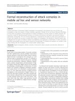
The fire-detection application scenario is summarized in Figure 1.1. We remark that this
scenario has several interesting features, such as reduced impact on the environment (since
sensor nodes have wireless transceivers, no wiring is needed), accuracy of coverage, and
prompt alerting of the human operator.
The above-described example outlines the features of a typical WSN application
scenario:
– Homogeneous network : Differing from the case of ad hoc networks, a WSN is typ-
ically composed of nodes with the same features, especially for what concerns the
communication apparatus. A partial exception to this rule is when different types of
smart sensor nodes are used in the same network: for instance, a few ‘super nodes’
(with more memory and/or with a longer transmitting range) could be used in combina-
tion with standard sensor nodes to increase the network monitoring ability. However,
also in this case the number of different device classes used in the network is very
limited (2–3 at most).
Figure 1.1 Sensor network used for prompt fire detection. When a fire is detected, an alarm
message (arrow) is generated by the sensor node(s) that detected the fire. The message is
then propagated in the network until it reaches a park ranger.

AD HOC AND SENSOR NETWORKS 7
Table 1.1 Comparison of typical features of
wireless ad hoc and sensor networks
Ad hoc Networks WSNs
Heterogeneous devices Homogeneous devices
Mobile nodes Stationary nodes
Dispersed network Dispersed network
Large network size
– Stationary or quasistationary network : Differing from the case of ad hoc networks,
nodes composing a WSN are typically stationary, or at most slowly moving. Given
the very wide range of WSN applications, exceptions to this rule are possible. This
is the case, for instance, of a sensor network used to track animal movements.
– Relatively dispersed network : this feature is in common with ad hoc networks: a
wireless sensor network is typically formed by nodes that are dispersed in a relatively
large geographical region, so that 1-hop communication between nodes is, in general,
not possible.
– Large network size: Typically, the number of nodes composing a WSN is quite large,
ranging from few tens to thousands of nodes.
The differences/similarities between ad hoc and sensor networks are summarized in
Table 1.1.
Among the many possible WSN application scenarios, we cite the following:
– Ocean temperature monitoring for improved weather forecast: It is known that the
evolution of weather conditions is strongly influenced by the temperature of large
water masses such as the oceans. However, nowadays our ability to perform a large-
scale monitoring of the ocean temperature is scarce. Sensor networks can be used
for this purpose. By dropping a large number of tiny sensors into the sea, water
temperature and ocean currents can be accurately monitored, helping the scientists in
the task of providing more accurate weather forecast.
– Intrusion detection: Camera-equipped sensors can be used to form a network that
monitors an area with restricted access. If the network is properly deployed, intruders

can be detected and an alarm message quickly propagated to the external observer.
– Avalanche prediction: Sensors equipped with location devices (such as GPS) can be
used to monitor the movements of large snow masses, thus allowing a more accurate
avalanche prediction.
1.2 Challenges
Although the technology for ad hoc and sensor networks is relatively mature, the applications
are almost completely lacking. This is in part due to the fact that some of the problems
8 AD HOC AND SENSOR NETWORKS
related to ad hoc/sensor networking are still unsolved. In this section, we describe the state
of progress of the current ad hoc and sensor network technology, and the main challenges
that face the ad hoc/sensor network designer.
1.2.1 Ad hoc networks
Wireless ad hoc networks have attracted the attention of researchers in academia and industry
in the last few years. As a result of this considerable research activity, the basic mechanisms
that enable wireless ad hoc communication have been designed and standardized. Just to
cite the most popular examples, IEEE 802.11 (IEEE 1999) and Bluetooth (Bluetooth 1999)
are communication standards that are implemented in a variety of commercial wireless
equipment, and that allows infrastructure-less wireless communication between mutually
compliant devices. Thus, wireless, multihop communication between different types of
devices such as cell phones, laptops, PDAs, smart appliances, and so on, is possible with
currently available technology.
Despite the fact that the technology for ad hoc network exists, applications based on the
ad hoc networking paradigm are almost completely lacking. This is because many of the
challenges to be faced for a practical implementation of ad hoc network services are still to
be solved. The main such challenges are the following:
– Energy conservation: Since units in ad hoc networks are typically battery equipped,
one of the primary design goals is to use this limited amount of energy as efficiently
as possible.
– Unstructured and/or time-varying network topology: Since the network nodes can,
in principle, be arbitrarily placed in a certain region and are typically mobile, the

topology of the graph that represents the wireless communication links between the
nodes is usually unstructured. Furthermore, the network topology may vary with
time, because of node mobility and/or failure. In these conditions, optimizing the
performance of ad hoc network protocols is a very difficult task.
– Low-quality communications: Communication on a wireless channel is, in general,
much less reliable than in a wired channel. Furthermore, the quality of communica-
tion is influenced by environmental factors (weather conditions, presence of obstacles,
interference with other radio networks, etc.), which are time varying. Thus, applica-
tions for ad hoc networks should be resilient to dramatically varying link conditions,
tolerating also nonnegligible off-service time intervals of the wireless link.
– Resource-constrained computation: Ad hoc networks are characterized by scarce
resource availability; in particular, energy and network bandwidth are available in
very limited amounts as compared to more traditional network paradigms. Protocols
for ad hoc networks must strive to provide the desired performance level in spite of
the few available resources.
– Scalability: In some ad hoc network scenarios, the network can be composed of
hundreds or thousands of nodes. This means that protocols for ad hoc networking
must be able to operate efficiently in the presence of a very large number of nodes
also.
AD HOC AND SENSOR NETWORKS 9
In case of ad hoc networks used for ‘ubiquitous’ networking, the following issues must
also be addressed:
– Interoperability: In the ‘ubiquitous’ networking scenario described in Section 1.1.1,
data should travel through the most diverse type of networks: ad hoc, cellular, satellite,
wireless LAN, PSTN, Internet, and so on. Ideally, the user should smoothly switch
from one network to the other without interrupting her applications. Implementing
this sort of ‘network handoff’ is a very challenging task.
– Definition of a feasible business model : Currently, accounting in wireless networks
(cellular, and commercial wireless Internet access) is done at the base station, that
is, using a centralized infrastructure. Furthermore, roaming is allowed only within

networks of the same type (e.g. cell phone roaming when the user is in a foreign
country). In the ‘ubiquitous’ scenario, it is still not clear which infrastructure should
perform billing and which rules should be used to regulate roaming between different
types of networks.
– Stimulate cooperation between nodes: When designing a certain network protocol,
it is usually assumed that all the nodes in the network voluntarily participate in the
protocol execution. In some ad hoc network application scenarios, network nodes
are owned by different authorities (private users, professionals, profit and/or nonprofit
organizations, and so on), and voluntary participation in the protocol execution cannot
be taken for granted. Thus, network nodes must be somehow stimulated to behave
according to the protocol specifications. The issue of stimulating cooperation between
nodes is treated in some detail in Chapter 16.
1.2.2 Wireless sensor networks
In a manner similar to ad hoc networks, WSNs also have attracted the attention of both
the academic and the industrial research community in the last few years. Firstly, a number
of smart sensor prototypes have been designed and implemented by the academic research
community. The most famous of such prototypes are probably the Berkeley Motes (Polastre
et al. 2004) and Smart Dust (Pister 2001). Later on, many academic interdisciplinary projects
have been funded (and are currently being funded) to actually deploy and utilize sensor
networks. One such example is the Great Duck Island project, in which a WSN has been
deployed to monitor the habitat of the nesting petrels without any human interference with
animals (Mainwaring et al. 2002).
Smart sensor nodes are also being produced and commercialized by some electronic
manufacturer. We cite Crossbow, a company that produces on a large scale the Motes
sensor nodes developed at UC Berkeley. Other major silicon companies such as Intel,
Philips, Siemens, STMicrolectronics, and so on, are interested in the WSN technology, and
are developing their own smart sensor node platform.
There is also a considerable standardization activity in the field of WSNs. The most
notable effort in this direction is the IEEE 802.15.4 standard currently under development,
which defines the physical and MAC layer protocols for remote monitoring and control,

as well as sensor network applications. ZigBee (ZigBeeAlliance 2004) is an industry con-
sortium (currently involving more than 100 members, representing 22 countries on four
continents) with the goal of promoting the IEEE 802.15.4 standard.
10 AD HOC AND SENSOR NETWORKS
Currently, we are in a phase in which the technology for implementing wireless sen-
sor networks is relatively mature but applications based on sensor networks have not been
completely defined. In particular, industries strive to find significant markets for WSN appli-
cations. The most promising ones seem to be home control, building automation, industrial
automation, and automotive applications (ZigBeeAlliance 2004). Nevertheless, the market
for wireless sensor hardware is expected to grow at the rate of 20% per year in the next few
years, which is three times the growth rate of the wired sensor market (Frost and Sullivan
2003).
In case of sensor networks also, many challenges are still to be faced before they can
be deployed on a large scale. The main challenges related to WSN implementation are the
following:
– Energy conservation: If reducing node energy consumption is important in ad hoc
networks, it becomes vital in WSNs. In fact, because of the reduced sized of the
sensor nodes, the battery has low capacity, and the available energy is very limited.
Despite this scarcity of energy, the network is expected to operate for a relatively long
time. Given that replacing/refilling batteries is usually impossible, one of the primary
design goals is to use this limited amount of energy as efficiently as possible.
– Low-quality communications: Sensor networks are often deployed in harsh envi-
ronments, and sometimes they operate under extreme weather conditions. In these
situations, the quality of the radio communication might be extremely poor, and
performing the requested collective sensing task might become very difficult.
– Operation in hostile environments: In many scenarios, sensor networks are expected
to operate under critical environmental conditions. Thus, it is essential that in these
cases the physical sensor nodes are carefully designed. Furthermore, the protocols
for network operation should be resilient to sensor faults, which can be considered a
relatively likely event.

– Resource-constrained computation: If the resources in ad hoc networks are scarce,
the situation is even worse in WSNs. Protocols for sensor networks must strive to
provide the desired QoS in spite of the few available resources.
– Data processing: Given the energy constraints and the relatively poor communica-
tion quality, the data collected by the sensor node must be locally compressed, and
aggregated with similar data generated by neighboring nodes. This way, relatively few
resources are used to communicate the data to the external observer. Since the observer
is often interested in getting data with different levels of accuracy depending, for
instance, on the events currently going on in the monitored region, the data aggrega-
tion mechanism should be able to provide different levels of compression/aggregation,
addressing the data accuracy/resource consumption trade-off.
– Scalability: WSNs are typically composed of hundreds or even several thousands of
nodes. Thus, the scalability of protocols for WSNs must be explicitly considered at
the design stage.
– Lack of easy-to-commercialize applications: Nowadays, several chip makers and elec-
tronic companies have started the commercial production of sensor nodes. However,
AD HOC AND SENSOR NETWORKS 11
it is much more difficult for these companies to commercialize applications based
on sensor networks. Selling applications, instead of relatively cheap sensors, would
be much more profitable for industry. Unfortunately, most sensor network application
scenarios are very specific, and a company would have little or no profit in devel-
oping an application for a very specific scenario since the potential buyers would be
very few.

2
Modeling Ad Hoc Networks
In this chapter, we introduce a simple but widely accepted model of ad hoc network. Since
sensor networks are a subclass of ad hoc networks, this model applies to this type of
networks also.
2.1 The Wireless Channel

Nodes in ad hoc and sensor networks communicate through wireless transceivers. For this
reason, an important building block of any model for ad hoc networks is the wireless channel
model. The model presented in this section is based on the material contained in (Rappaport
2002).
A radio channel between a transmitter unit u and a receiver unit v is established if and
only if the power of the radio signal received by node v is above a certain threshold, called
the sensitivity threshold. Formally, there exists a direct wireless link between u and v if
P
r
≥ β,whereP
r
is the power of the signal received by v,andβ denotes the sensitivity
threshold. The exact value of β depends on the features of the wireless transceiver and on
the communication data rate: for a given radio, the higher the data rate, the higher the value
of β, implying a stronger requirement on the received power. In order to simplify notation,
in the following we assume that β has the conventional value of 1.
The received power P
r
depends on the power P
t
used by u to transmit the radio signal,
and on the path loss, which models the radio signal degradation with distance. Denoting
with PL(u, v) the path loss between units u and v, we can write
P
r
=
P
t
PL(u, v)
.

Thus, the occurrence of a radio channel between any two network nodes can be predicted
if the path loss model is known.
Modeling path loss has historically been one of the most difficult tasks of the wireless
system designer. The mechanisms that regulate radio signal propagation in the environment
can be grouped into three categories: reflection, diffraction and scattering. Reflection occurs
Topology Control in Wireless Ad Hoc and Sensor Networks P. Santi
 2005 John Wiley & Sons, Ltd
14 MODELING AD HOC NETWORKS
when the electromagnetic wave hits the surface of an object that has very large dimensions
when compared to the wavelength of the propagating signal. For instance, the radio signal
is reflected by the surface of the earth and by large buildings and walls. Diffraction is
caused by objects with very sharp edges that lie on the radio path between the transmitter
and the receiver. Scattering occurs when several small objects (as compared to the signal
wavelength) are in between the transmitter and the receiver of the radio signal. Typical
sources of scattering are foliage, street signs, and so on. Given these mechanisms, it is
clear that radio wave propagation is an extremely complex phenomenon, which is heavily
influenced by environmental factors. In the following, we shortly describe the most common
path loss models introduced in the literature. For a detailed treatment of this subject, the
reader is referred to (Rappaport 2002).
2.1.1 The free space propagation model
This model is used to predict radio signal propagation when the path between the transmitter
and the receiver is clear and unobstructed (line-of-sight, or LOS, path). Denoting with P
r
(d)
the power of the radio signal received by a node located at distance d from the transmitter,
we have
P
r
(d) =
P

t
G
t
G
r
λ
2
(4π)
2
d
2
L
, (2.1)
where G
t
is the transmitter antenna gain, G
r
is the receiver antenna gain, L is the system
loss factor not related to propagation, and λ is the wavelength in meters. Since we are not
interested in the specific characteristics of the transceiver, we can simplify equation (2.1)
as follows:
P
r
(d) = C
f
·
P
t
d
2

, (2.2)
where C
f
(f stands for free space) is a constant that depends on the characteristics of the
transceivers.
Equation (2.2) shows that the received power falloff is proportional to the square of the
distance d that separates the transmitter and the receiver. Combining equation (2.2) with the
sensitivity threshold, we can state that the transmitted message can be correctly received if
and only if
d ≤

C
f
P
t
.
In other words, the radio coverage area of a node transmitting at power P
t
is a disk of
radius
√
C
f
P
t
centered at the node.
The free space equation is valid only for values of d that are relatively far from the
transmitting antenna. For values of d within the so-called close-in distance d
0
, the path loss

can be assumed to be constant.
2.1.2 The two-ray ground model
It is seldom the case that the single direct path between the transmitter and the receiver
is the only physical means of propagation of the radio signal. For this reason, the free
space propagation model is often inaccurate. To improve accuracy, the two-ray ground
model considers two propagation paths: the directed path and a ground reflected propagation
between the transmitter and the receiver (see Figure 2.1).
MODELING AD HOC NETWORKS 15
u
v
d
h
t
h
r
Figure 2.1 The two-ray propagation model: the radio signal sent by node u reaches node
v through the direct path, and through a ground reflected path.
In the two-ray ground propagation model, the received power at distance d is given by
the following formula:
P
r
(d) = P
t
G
t
G
r
h
2
t

h
2
r
d
4
, (2.3)
where h
t
is the transmitter antenna height and h
r
is the receiver antenna height. If the
distance between the sender and the receiver is relatively large (d 
√
h
t
h
r
), and abstracting
the features of the radio transceivers, we can write the following simplified formula:
P
r
(d) = C
t
·
P
t
d
4
, (2.4)
where C

t
(t stands for two-ray ground) is a constant that depends on the characteristics of
the radio transceivers. So, the major difference with the free space model is that the radio
signal falloff in this case is proportional to the distance raised to the fourth power, instead
of to the square of the distance.
Combining equation (2.4) with the sensitivity threshold, we have that the radio coverage
region in the two-ray ground model is a disk of radius
4
√
C
t
P
t
centered at the transmitter.
2.1.3 The log-distance path model
The log-distance model has been derived combining analytical and empirical methods.
Empirical methods are based on field measurements and reverse curve fitting on the exper-
imental data.
This model, which can be seen as a generalization of both the free space and the two-
ray ground model, indicates that the average long-distance path loss is proportional to the
separation distance d raised to a certain exponent α, which is called the path loss exponent ,
or distance-power gradient. Formally,
P
r
(d) ∝
P
t
d
α
. (2.5)

The radio coverage region in this model is a disk of radius proportional to
α
√
P
t
centered
at the transmitter.
The value of α depends on the environmental conditions, and it has been experimentally
evaluated in many scenarios. Table 2.1 summarizes some of these values.
16 MODELING AD HOC NETWORKS
Table 2.1 Values of the
distance-power gradient in
different environments
Environment α
Free space 2
Urban area 2.7–3.5
Indoor LOS 1.6–1.8
Indoor no LOS 4–6
2.1.4 Large-scale and small-scale variations
The log-distance propagation model predicts the average received power at a certain dis-
tance. However, the intensity of the received signal can vary a lot from the average value.
For this reason, probabilistic models have been used to account for the variability of the
wireless channel. In a probabilistic propagation model, the radio coverage region is no
longer a disk, since the occurrence of a wireless channel between two nodes is a random
event.
Probabilistic propagation models can be divided into two classes:
– Large-scale models: These models predict variations of the signal intensity over large
distances.
– Small-scale models: These models predict variations of the signal intensity over very
short distance. They are also called multipath fading (or simply fading) models.

The most important large-scale model is the log-normal shadowing model, in which the
path loss at distance d is modeled as a random variable with log-normal distribution (see
Appendix B for a definition of log-normal distribution) centered about the mean value, which
is stated in equation (2.5). The most important fading model is the Rayleigh model, which
models small-scale variations of the radio signal intensity according to a random variable
with Rayleigh distribution. A detailed description of probabilistic radio propagation models
can be found in (Rappaport 2002).
2.2 The Communication Graph
The communication graph defines the network topology, that is, the set of wireless links
that the nodes can use to communicate with each other. Given the discussion of the previous
section, it is clear that the presence of a link between two units u and v in the network
depends on (i) the relative distance between u and v, (ii) the transmit power used to send
the data, and (iii) the surrounding environment. Since accounting for large- and small-
scale variations of the radio signal is quite complicated, and renders the link model tightly
coupled with a specific application scenario, in this section and in the rest of this book we
will model the wireless channel using the log-distance path model, which abstracts many
characteristics of the environment. This assumption is standard in research on topology
control in ad hoc/sensor networks.
MODELING AD HOC NETWORKS 17
Let N be a set of wireless nodes, with |N|=n. These nodes are located in a certain
bounded region R. For simplicity, we assume that R is a d-dimensional cube of side l.
Formally, R = [0,l]
d
for some l>0, where d = 1, 2, 3. For any u ∈ N,thelocation of
u in R, denoted L(u), is the position of u in R, expressed as d-dimensional coordinates.
Thus, function L : N → R maps every node of the network to its physical location within
R. If nodes are mobile, the physical node location is time dependent. If nodes move within
R – we can assume this without loss of generality – mobility can be represented by adding a
further argument to L, the time instant t. Summarizing, function L : N × T → R assigns to
every element of N and to any time t ∈ T asetofd-dimensional coordinates, representing

the physical node’s location at time t.Ad-dimensional mobile ad hoc network is then
represented by the pair M
d
= (N, L),whereN and L are defined as above.
Given a network M
d
= (N, L),arange assignment for M
d
is a function RA that assigns
to every element u of N avalueRA(u) ∈ (0,r
max
], representing its transmitting range.
Parameter r
max
is called the maximum transmitting range, and depends on the features of
the radio transceivers equipping the nodes. It is usually assumed that network nodes are
equipped with transceivers having similar features, that is, r
max
is the same for all the nodes
in the network. In case the network is composed of units equipped with transceivers of
different type, r
max
is intended as the maximum over the transmitting ranges of the different
radios, and the definition of transmitting range is still sound.
The transmitting range of a node u denotes the range within which the data transmitted
by u can be correctly received. Given the range r, the definition of the subregion of R
within which correct data reception is possible depends on the network dimension: in case
of one-dimensional networks, it is the segment of length 2r centered at u; in case of
two-dimensional networks, it is the circle of radius r centered at u; in three-dimensional
networks, it is the sphere of radius r centered at u (see Figure 2.2).

Note that, under the assumption that the radio signal propagates according to the log-
distance path model, any transmitting range r ∈ (0,r
max
] is uniquely associated with a
transmit power P
r
∈ (0,P
max
], where P
max
is the maximum transmit power level of the
nodes. Thus, the notions of node’s transmitting range and node’s transmit power are equiv-
alent, and they will be interchangeably used in the rest of this book.
Given a network M
d
= (N, L) and a range assignment RA,thecommunication graph
induced by RA on M
d
at time t is defined as the directed graph G
t
= (N, E(t)),
where the directed edge [u, v] exists if and only if RA(u) ≥ δ(L(u,t),L(v,t)),where
δ(L(u,t),L(v,t)) is the Euclidean distance between u and v at time t.Inotherwords,
the directed wireless link (u, v) exists if and only if nodes u and v are at distance of at most
u
rr
u
(a) (b) (c)
r
u

r
Figure 2.2 Radio coverage in one-dimensional (a), two-dimensional (b), and three-
dimensional (c) networks. The covered region has radius r, and it is centered at the unit.
18 MODELING AD HOC NETWORKS
RA(u) at time t. In this case, v is said to be a 1-hop neighbor, or neighbor for short, of
node u. A wireless link is said to be bidirectional,orsymmetric, at time t if (u, v) ∈ E(t)
and (v, u) ∈ E(t). In this case, nodes u and v are said to be symmetric neighbors.
The maxpower range assignment is such that RA(u) = r
max
for every node u,thatis,
every node in the networks transmits at maximum power. The resulting communication
graph is called the maxpower graph, and represents the set of all possible communication
links between the network nodes.
A range assignment RA is said to be connecting at time t, or simply connecting,ifthe
resulting communication graph at time t is strongly connected, that is, if for any pair of
nodes u and v, there exists at least one directed path from u to v. A range assignment
in which all the nodes have the same transmitting range r, for some 0 <r≤ r
max
,is
called r-homogeneous. When the exact value of r is not relevant, the r-homogeneous range
assignment is simply called homogeneous. Observe that the communication graph generated
by a homogeneous range assignment can be considered as undirected, since (u, v) ∈ E(t) ⇔
(v, u) ∈ E(t).
If the network is mobile, the range assignment may vary with time in order to preserve
a certain property of the communication graph, such as connectivity. In general, we can
then define a sequence of range assignments RA
t
1
, RA
t

2
, during the network lifetime,
where RA
t
i
is the range assignment at time t
i
, and the transition between range assignments
is determined by an appropriate protocol.
If the network is stationary (i.e. the position of every node does not change during the
entire network operational lifetime), the model described above can be simplified by making
L a function of N only. Nevertheless, different range assignments can, in principle, be used
during the network lifetime. The range assignment can be varied, for instance, to support
different kinds of traffic (for example, in a sensor network, the type of information delivered
to the external observer changes depending on the detected events), or to achieve a balanced
energy consumption among network nodes. Thus, in general, the communication graph is
time dependent even if the network is stationary.
The model described in this section is essentially the point graph model introduced in
(Sen and Huson 1996). An example of two-dimensional point graph is reported in Figure 2.3.
Similar graph models have been used in applied probability theories, such as continuum per-
colation and geometric random graphs. In the former theory, a unit disk graph is a graph
in which every two nodes are connected with an edge if and only if they are at distance
at most 1. Up to a normalization, unit disk graphs correspond to the model described in
this section with homogeneous range assignment. In the theory of GRG, a set of points is
distributed according to some probability distribution in a certain region. Points are then con-
nected according to some rule (e.g. connect to all the points within distance r, or connect to
the k closest nodes, etc.), generating a geometric random graph. Also, this model is a special
case of ours, in which it is assumed that nodes are randomly distributed and that the range
assignment is defined by a specific rule. The interested reader can find additional information
on the theories of continuum percolation and of geometric random graphs in Appendix B.

The main weakness of the point graph model is the assumption of perfectly regular
radio coverage: the covered region is a d-dimensional disk of a certain radius centered at
the transmitter. As discussed in the previous section, this assumption is quite realistic in
open air, flat environments. Unfortunately, ad hoc and sensor networks are likely to be used
in very different situations, such as indoor or urban scenarios (ad hoc networks), or under
MODELING AD HOC NETWORKS 19
Figure 2.3 Example of two-dimensional point graph. Note that two of the links in the graph
are unidirectional.
harsh conditions (sensor networks). In other words, in real-life situations, it is quite likely
that the radio coverage region is highly irregular, because of the influence of walls, buildings,
interference with preexisting infrastructure, and so on. However, including all these details in
the network model would make it extremely complex and scenario dependent, hampering the
derivation of meaningful and sufficiently general analytical results. For this reason, despite its
limitations, the point graph model is widely used in the study of ad hoc network properties.
Before ending this section, we want to emphasize that the results obtained using the point
graph model are useful, at least to some extent, also in situations in which the radio coverage
region is known to be irregular. For instance, suppose we want to formally characterize the
minimum value of r such that the r-homogeneous range assignment is connecting. If the
network is two-dimensional, the value of r thus obtained can be thought of as the radius
of the largest circular subarea of the actual radio coverage area. Thus, there could exist
nodes that are 1-hop neighbors in reality, but that are not directly connected in the point
graph model. It follows that the actual network connectivity is higher than that formally
characterized using the point graph model. Clearly, the analytical characterization of r
becomes less and less significant from a practical point of view as the actual radio coverage
area is more and more irregular.
2.3 Modeling Energy Consumption
One of the primary concerns of the ad hoc/sensor networks designer is the efficient use of
energy. Thus, it is fundamental to model the node energy consumption accurately. Since
20 MODELING AD HOC NETWORKS
the features of typical nodes in ad hoc and sensor networks are quite different, we discuss

energy models for the two classes of networks separately.
2.3.1 Ad hoc networks
Depending on the scenario, ad hoc networks can be composed of nodes of the most diverse
type: laptops, cellular phones, PDAs, smart appliances, and so on. Furthermore, for many
application scenarios (e.g. the ‘ubiquitous network’), the network can be composed of het-
erogeneous devices. Given this node diversity, a typical approach in the literature is to
focus attention on the energy consumption of the wireless transceiver only. This is also our
choice, which is further motivated by the fact that topology control is primarily concerned
with reducing the energy consumed to communicate.
Depending on the type of device, the amount of energy consumed by the transceiver
varies from about 15 to about 35% of the total energy dissipated by the node. The former
value refers to a laptop equipped with a IEEE 802.11 wireless card, while the latter is typical
of a PDA device. Since the energy consumed by the wireless card is a significant portion
of the total power dissipation in the node, optimizing the energy used to communicate is an
important issue.
Several authors have measured the energy consumption of commercial 802.11 wireless
cards. Typically, an IEEE 802.11 wireless card has four operational modes:
– Idle: The radio is turned on, but it is not used.
– Transmit: The radio is transmitting a data packet.
– Receive: The radio is receiving a data packet.
– Sleep: The radio is powered down.
Table 2.2 shows the power consumption of a CISCO Aironet IEEE 802.11 a/b/g card, as
reported in the data sheets (Cisco 2004). Power consumption in sleep mode is not reported
in the data sheets. The table also reports the nominal transmitting ranges when the card
transmits at full power. As seen from the table, the nominal range depends on environmental
factors (indoor or outdoor conditions) and on the data rate used to send the message.
We remark that the data reported in Table 2.2 are nominal, and can be considerably
different from the actual power consumption of the wireless card. For instance, if we consider
the specifics of the CISCO Aironet 350 card as reported in the data sheets, the sleep : idle :
rx : tx power ratios are 0.07:1:1.33:2.22 (Cisco 2004). These values must be compared with

the ratios computed with the measured power consumption, which are 0.04:1:1.20:1.73 (see
(Shih et al. 2002)). Measurements performed on other models of IEEE 802.11 wireless
cards can be found in (Ebert et al. 2002; Feeney and Nilsson 2001). All the measurements
reported in the literature have outlined an important point, that is, that any radio state
transition comes at a significant energy cost (and time latency). This is especially true when
the radio transits from the sleep (power down) to the idle (power up) state.
In this book, we model node energy consumption by using the sleep : idle : rx : tx power
ratios. In other words, we are not interested in the absolute values of the power consumption,
but on the relative values. In our simplified model, we assume that the radio is consuming
conventional power 1 when the radio is idle, power 1.x when the radio is receiving a
MODELING AD HOC NETWORKS 21
Table 2.2 Nominal power consumption and transmit range of the CISCO IEEE
802.11 a/b/g wireless card. Power consumption is measured by the drain current,
expressed in mA. In the table, the minimum value of the nominal range refers to
the maximum data rate (54 Mbps), and the maximum value to the 6 Mbps data
rate
Power Idle (mA) Power Tx (mA) Power Rx (mA)
802.11 a 203 554 318
802.11 b 203 539 327
802.11 g 203 530 282
Tx Range Indoor (m) Tx Range Outdoor (m)
802.11 a 13–50 30–300
802.11 b/g 27–91 76–396
message, power 1.y when the radio is transmitting a message at full power, and power
0.z when the radio is in sleep mode (the actual values of x, y,andz depending on the
specific card).
Before ending this section, we want to remark that the ratio 1.y used in our model refers
to the relative power consumption of the radio when it transmits at maximum power. On
the other hand, we shall see that topology control protocols are based on the ability of the
wireless node to dynamically adjust its transmitting range. This feature is actually available

on some commercial IEEE 802.11 cards, such as those produced by CISCO. For instance,
the CISCO Aironet IEEE 802.11 a/b/g card can use transmit powers ranging from 1 mW to
100 mW. However, this value refers to the power consumption of the RF amplifier, which
is only a part of the total power consumed by the wireless card. In fact, the card consumes
significant energy also to power up the other analog and digital circuitry.
How to model power consumption when the radio is not transmitting at maximum
power is not clear. Most of the approaches presented in the literature are concerned with
the transmit power only, which is typically modeled using one of the formulas reported in
Section 2.1. Unless otherwise specified, this book will also follow this simplistic energy
model. In particular, we will use the following definition of energy cost:
Definition 2.3.1 (Energy cost) Given a range assignment RA for a certain network M
d
=
(N, L), the energy cost of RA is defined as
c(RA) =

u∈N
RA(u)
α
,
where α is the distance-power gradient.
Note that the above definition of energy cost is coherent with our working assumption
that the radio signal propagates according to the log-distance path model.
2.3.2 Sensor networks
In case of sensor networks, the task of providing a simple yet realistic energy model is
relatively simpler, as compared to the case of ad hoc networks. In fact, sensor networks are
22 MODELING AD HOC NETWORKS
Table 2.3 Measured power consumption of a Rockwell’s WINS sensor node
MCU Mode Sensor Mode Radio Mode Total Power (mW)
On On Tx (power 36.3 mW) 1080.5

On On Tx (power 0.12 mW) 771.1
On On Rx 751.6
On On Idle 727.5
On On Sleep 416.3
On On Removed 383.3
Sleep On Removed 64.0
typically composed of homogeneous devices, which are usually very simple. Furthermore,
since many sensor nodes have been designed in the research community, their features are
very well known. As a result, several sets of energy consumption measurements of wireless
sensor nodes have been reported in the literature (Raghunathan et al. 2002).
Table 2.3 reports the power dissipation of a Rockwell’s WINS sensor node (Rock-
wellScienceCenter 2004). The node is composed of three main components: the microcon-
troller unit (MCU), the sensing apparatus (sensor), and the wireless radio. If we consider the
power consumption of the wireless radio only, we have the following sleep : idle : rx : tx
ratios: 0.09:1:1.07:2.02. Note that these ratios are quite similar to the case of 802.11 wireless
cards, except for a somewhat higher power consumption when the radio is transmitting at
maximum power. When the transmit power is minimum (0.12 mW), the idle : tx ratio in the
WINS sensor is 1.12. So, there is an almost twofold power consumption increase when vary-
ing the transmit power from the minimum to the maximum value. This means that varying
the transmit power level has a considerable effect on the node’s energy consumption.
2.4 Mobility Models
Node mobility is a prominent feature of ad hoc networks and, in some cases, also of WSNs.
As a consequence, studying the performance of ad hoc/sensor networking protocols in the
presence of mobility is a fundamental stage of the design process. Since real implementations
of ad hoc/sensor networks are scarce, real-life movement patterns are very difficult to obtain,
and the common approach is to use synthetic mobility models and simulation.
Mobility models for ad hoc/sensor networks should
– resemble real-life movements: Given the wide range of ad hoc and sensor network
applications, the movement patterns to consider are numerous: they range from cam-
puswide movement of students to vehicular motion in highways, from movement of

groups of tourists in a urban scenario to rescue squads motion in disaster areas, and
from sensors carried around by ocean flows to animal movement in animal tracking
WSN applications. Providing a unique mobility model that resembles all these types of
mobility is virtually impossible. However, a mobility model should be representative
of at least one application scenario.
– be simple enough for simulation/analysis: Since mobility models are used in the sim-
ulation of ad hoc networks, the model should be simple enough to be integrated in the
MODELING AD HOC NETWORKS 23
simulator and to keep the simulation running time reasonable. Furthermore, using rel-
atively simple mobility models eases the task of deriving meaningful analytical results
concerning fundamental network parameters in presence of mobility. In turn, these
results can be used to optimize the performance of ad hoc/sensor networking protocols.
Clearly, the two goals above are conflicting: the more realistic the model is, the more
the details that must be included in it, and the model complexity increases. Thus, a synthetic
mobility model should be a good compromise between representativeness and simplicity, that
is, it should consider the salient features of a certain movement pattern, while disregarding
secondary details.
In this section, we briefly describe the most important mobility models used in the
simulation of ad hoc/sensor networks. For a more detailed description of mobility models
for ad hoc networks, see (Bettstetter 2001a; Camp et al. 2002).
Random waypoint model. This is by far the most commonly used mobility model for
ad hoc networks. One of the reasons for its popularity is the fact that it is implemented in
network simulations tools such as Ns2 (Ns2 2002) and GloMoSim (Zeng et al. 1998). The
Random Waypoint (RWP) model has been introduced in (Johnson and Maltz 1996) to study
the performance of the DSR routing protocol. In this model, each node chooses uniformly
at random a destination point (the ‘waypoint’) within the deployment region R, and moves
toward it along a straight line. Node velocity is chosen uniformly at random in the interval
[v
min
,v

max
], where v
min
and v
max
are the minimum and maximum node velocities. When
the node arrives at destination, it remains stationary for a predefined pause time, and then
starts moving again according to the same pattern.
The RWP model is representative of an individual movement, obstacle-free scenario:
each node moves independent of each other (individual movement), and it can potentially
move in any subregion of R (obstacle-free). For instance, a similar type of mobility could
arise when users move in a large room, or in a open air, flat environment.
Given its popularity, RWP mobility has been deeply studied in the literature. In particular,
it has been recently discovered that the long-term node spatial distribution of RWP mobile
networks is concentrated in the center of the deployment region (border effect) (Bettstetter
and Krause 2001; Bettstetter et al. 2003; Blough et al. 2004), and that the average nodal
speed, defined as the average of the node velocities at a given instant of time, decreases over
time (Yoon et al. 2003). These observations have brought to the attention of the community
the fact that RWP mobile networks must be carefully simulated. In particular, network
performance should be evaluated only after a certain ‘warm-up’ period, which must be
long enough for the network to reach the node spatial and average velocity ‘steady-state’
distribution.
The RWP model has also been generalized to slightly more realistic, though still simple,
models. For instance, in (Bettstetter et al. 2003) the RWP model is extended by allow-
ing nodes to choose pause times from an arbitrary probability distribution. Furthermore, a
random fraction of the network nodes remains stationary for the entire simulation time.
Random direction model. Similar to the RWP model, the random direction model resem-
bles individual, obstacle-free movement. This model was created to maintain a uniform node
spatial distribution during the simulation time, thus avoiding the border effect typical of RWP
mobility.

24 MODELING AD HOC NETWORKS
In this model (Royer et al. 2001), any node chooses a direction uniformly at random in
the interval [0, 2π], and a random velocity in the interval [v
min
,v
max
]. Then, it starts moving
in the selected direction with the chosen velocity. When the node reaches the boundary of
R, it chooses a new direction and velocity, and so on.
Variants of this model have also been presented. In a first variant (Haas and Pearlman
1998; Pearlman et al. 2000b), a node is ‘bounced back’ when it reaches the boundary
of the deployment region. In another (Bettstetter 2001b), the node moves for a random
(exponentially distributed) time, and then it changes direction and velocity of movement.
Brownian-like motion. Contrary to the case of RWP and random direction mobility,
which resemble intentional movement, the class of Brownian-like mobility models resembles
nonintentional motion. For this reason, these models are sometimes called drunkardlike
models.
In Brownian-like motion, the position of a node at a given time step depends (in a
certain, probabilistic, way) on the node position at the previous step. In particular, no
explicit modeling of movement direction and velocity is used in this model.
An example of Brownian-like motion is the model used in (Santi and Blough 2003).
Mobility is modeled using three parameters: p
stat
, p
move
and m. The first parameter represents
the probability that a node remains stationary for the entire simulation time. Parameter p
move
is the probability that a node moves at a given time step. Parameter m models, to some
extent, velocity: if a node is moving at step i, its position at step i + 1 is chosen uniformly

at random in the square or side 2m centered at the current node position.
Map-based mobility. In all the models introduced so far, nodes are free to move within
any subregion of the deployment region R. However, in many realistic scenarios, nodes are
constrained to move within specified paths. This is the case, for instance, of cars moving on
a freeway, or people moving on sidewalks, and so on. Map-based models have been used
to model these situations.
The first step in the definition of map-based models is the map setup, that is, the
definition of the paths within which nodes are allowed to move. Then, a certain number of
nodes are randomly located on the paths, and they start moving according to scenario-specific
rules.
An instance of map-based mobility is the Freeway mobility model (Bai et al. 2003),
used to mimic the movement of cars on freeways. In this model, several freeways are
located in the deployment region. Each freeway is composed of a varying number of lanes
in both directions. Nodes are randomly located on a freeway, and they move with a random
velocity, which is temporally dependent on its previous velocity. If two nodes on the same
lane are within a certain minimum distance (safety distance), the velocity of the following
node cannot exceed the velocity of the preceding one.
Another instance of map-based mobility is the Manhattan mobility model (Bai et al.
2003), which is used to emulate urban movement scenarios. First, a Manhattan-like map,
composed of horizontal and vertical streets, is generated. Nodes can move along the streets
in both directions. When a node arrives at an intersection, it randomly chooses whether to
continue moving along the same direction, or to take a left or a right turn. Similar to the
Freeway model, the velocity of a node at a certain instant of time depends on the node
velocity at the previous time step.