Topology Control in Wireless Ad Hoc and Sensor Networks phần 4 pot

56 THE CTR FOR CONNECTIVITY: MOBILE NETWORKS
u
A
2
A
1
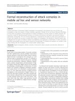
Figure 5.1 The border effect in RWP mobile networks: when a node is resting close to
the border, it is likely that the trajectory to the next waypoint crosses the center of the
deployment region (dark shaded area). In the figure, the probability that the trajectory of
node u to the next waypoint intersects A
1
equals the sum of the areas of A
1
and A
2
(we
are assuming R = [0, 1]
2
).
resting at a waypoint that is close to the border of R (see Figure 5.1). Since the next
waypoint is chosen uniformly at random in R, it is very likely that the trajectory connecting
node u with its next waypoint will cross the center of R. So, the probability of finding
a mobile node close to the center of R is higher than the probability of finding the node
on the boundary. This means that mobile nodes contribute a nonuniform component to the
asymptotic node spatial distribution generated by RWP mobility, which we denote by F
m
(m stands for ‘mobile’). On the other hand, a node resting at a waypoint contributes a
uniform component F
u
to the asymptotic RWP distribution, since the waypoints are chosen
uniformly at random in R. Then, the asymptotic node spatial distribution generated by

RWP mobility, denoted by F
RWP
,isgivenbyF
RWP
= F
m
+ F
u
, which is nonuniform. The
amount of this nonuniformity (and, hence, the intensity of the border effect) depends on
the relative strength of the two components of F
RWP
. It is easy to see that a longer pause
time strengthens F
u
, since the nodes remain stationary for a longer time. Conversely, F
m
is maximal when the pause time is 0 because, in this case, nodes are constantly moving.
The informal argument above is theoretically supported by the following theorem proven
in (Bettstetter et al. 2003), which derives a very good approximation of F
RWP
when nodes
move in R = [0, 1]
2
.
Theorem 5.1.1 (Bettstetter et al. 2003) The asymptotic spatial density function of a node
moving in R = [0, 1]
2
according to the RWP model with pause time t
p

and velocity v is
closely approximated by
F
RWP
(x, y) =

P
pause
+ (1 −P
pause
)F
m
(x, y) if(x, y) ∈ [0, 1]
2
0otherwise
,
THE CTR FOR CONNECTIVITY: MOBILE NETWORKS 57
where P
pause
=
t
p
t
p
+
0.521405
v
and
F
m

(x, y) =

0if(x = 0) or (y = 0)
F
R
(x, y) otherwise
.
The expression of F
R
(x, y) is the following:
F
R
(x, y) =
6y +
3
4
(1 − 2x + 2x
2
)

y
y − 1
+
y
2
(x − 1)x

+
3
2


(2x − 1)y(1 +y) log

1 −x
x

+ y(1 − 2x + 2x
2
+ y)log

1 −y
y

.
We remark that the expression of F
m
(x, y) above is valid only for (x, y) ∈ R ={(x, y) ∈
[0, 1]
2
|(x ≥ y) ∧ (x ≤ 1/2)}. The expression of F
m
(x, y) on the remainder of [0, 1]
2
can
be easily obtained observing that by symmetry we have F
m
(x, y) = F
m
(y, x) = F
m

(1 −
x,y) = F
m
(x, 1 −y).
The 3D plot of F
RWP
for different values of the pause time is reported in Figure 5.2:
as predicted by Theorem 5.1.1, longer pause times generate a flatter probability density
function.
The CTR in presence of RWP mobility can be characterized by using the following
result of the GRG theory, which is due to Penrose (Penrose 1999c).
Theorem 5.1.2 (Penrose 1999c) Assume n nodes are distributed independently at random
in R
2
according to a common probability density function F , having connected and compact
support  with smooth boundary ∂. Further, assume that F is continuous on ∂.LetM
n
denote the length of the longest MST edge built on the n points. Then,
lim
n→∞
nπ
(
M
n
)
2
log n
=
1
min


F
, (5.2)
almost surely.
t
p
=0
(a) (b) (c)
t
p
=75 t
p
= 150
Figure 5.2 3D plot of F
RWP
for three different values of t
p
: t
p
= 0(a),t
p
= 75 time steps
(b), and t
p
= 150 time steps (c). Velocity v is set to 0.01 units per time step.
58 THE CTR FOR CONNECTIVITY: MOBILE NETWORKS
We recall that the support  of a probability density function is the set of points in
which it has nonzero value, and that the boundary ∂ is smooth if and only if it is twice
differentiable.
Informally speaking, Theorem 5.1.2 states that the asymptotic behavior of the CTR

for connectivity with arbitrary density F depends only on the minimum value of F in its
support. In case min

F = 0, the limit in equation (5.2) must be intended as +∞.
In order to apply Theorem 5.1.2 to F
RWP
, we have to check that all the conditions of
the theorem are satisfied. It is immediate to see that R = [0, 1]
2
, the support of F
RWP
,is
connected and compact. However, the boundary ∂R of R is not smooth because of the
presence of the corners. This problem can be circumvented by using the ‘corner-rounding’
technique described in (Santi 2005). Thus, we are in the hypotheses of Theorem 5.1.2, and
the only thing left to do to characterize the CTR is to determine the minimum value of
F
RWP
in R. This can be easily done, given the expression of F
RWP
introduced in Theorem
5.1.1.
Corollary 5.1.3 Let F
t
p
RWP
denote the asymptotic node spatial density generated by RWP
mobile networks with pause time t
p
and velocity v. The minimum value of F

t
p
RWP
is achieved
on ∂R, and it equals P
pause
=
t
p
t
p
+
0.521405
v
. When t
p
→∞, F
t
p
RWP
becomes the uniform distri-
bution on [0, 1]
2
, and min
R
F
∞
RWP
= 1.
We are now ready to characterize the CTR in presence of RWP mobility.

Theorem 5.1.4 (Santi (2005)) If R = [0, 1]
2
and n nodes move in R according to the RWP
mobility model with pause time t
p
and velocity v, then the CTR for connectivity is
r
t
p
RWP
=
1
P
pause

log n
πn
=
t
p
+
0.521405
v
t
p

log n
πn
if t
p

> 0. When t
p
= 0, we have
r
0
RWP


log n
n
a.a.s.
Note that the CTR in presence of RWP mobility is always larger than the CTR in
case of uniform node distribution since 1/P
pause
is larger than 1 for any value of t
p
.For
instance, with t
p
= 75 and v = 0.01, we have 1/P
pause
= 1.69485. Clearly, a longer pause
time results in a more uniform node distribution and, consequently, in a smaller value of
the CTR. For instance, with t
p
= 150, we have 1/P
pause
= 1.34743.
Note also the asymptotic gap of the CTR in the most extreme case of RWP mobility,
that is, when t

p
= 0: in this case, for any constant c>0, setting the transmitting range to
c

log n
n
is not sufficient for achieving a.a.s. connectivity. The exact value of the CTR with
RWP mobility when t
p
= 0 is not known to date. In (Santi 2005), it is conjectured that
r
0
RWP
≈
1
4
log n

log n
πn
.
This formula is supported by experimental evidence.
THE CTR FOR CONNECTIVITY: MOBILE NETWORKS 59
Pause time = 75
0
0.1
0.2
0.3
0.4
0.5

0.6
0.7
10 100 1000 10 000
n
CTR
Exp CTR
Th CTR
Figure 5.3 CTR for connectivity in case of RWP mobility with t
p
= 75 and v = 0.01, for
increasing values of n. The lower plot (ThCTR) refers to the asymptotic value, calculated in
accordance with Theorem 5.1.4. The upper plot (ExpCTR) is obtained from the experimental
CTR distribution generated by the simulations.
Figure 5.3 shows the rate of convergence of the actual CTR for connectivity to the
asymptotic value stated in Theorem 5.1.4 in case of RWP mobility with t
p
= 75. The actual
CTR value is computed as follows. Initially, n nodes are distributed uniformly at random in
R = [0, 1]
2
. Then, they start moving according to the RWP mobility model. After a large
number of mobility steps (1000 in our experiments), nodes’ positions are recorded, and
utilized to generate the experimental distribution of the longest MST edge length in case of
mobility. As in the case of stationary networks, the experimental CTR value is defined as
the 0.99 quantile of this distribution.
From the Figure, it is seen that the formula of Theorem 5.1.4 is quite accurate only
for large values of n (n = 1000 and above). The experimental value of the CTR for RWP
mobile networks with different values of the pause time is reported in Table 5.1.
Before concluding this section, we prove that the RWP mobility model satisfies the
conditions for ergodicity.

Theorem 5.1.5 A network with RWP mobility is ergodic with respect to the CTR for con-
nectivity.
Proof. In order to prove the theorem, we have to show that the RWP mobility model
is stable and c-independent, for some constant c>0. The first property is an immediate
consequence of Theorem 5.1.1. As for the second, consider an arbitrary time instant i.We
have to determine a certain value c>0 such that the positions of all the nodes at time
i + c are independent of node positions at time i. Let us define a movement epoch as the
time needed for a node just arrived at a waypoint to reach the next waypoint. In other
words, a movement epoch is composed of the pause time plus the travel time between two
consecutive waypoints. Since the length of the trajectory and node velocity are in general
60 THE CTR FOR CONNECTIVITY: MOBILE NETWORKS
Table 5.1 Values of the transmitting range
yielding 99% of connected communication
graphs in RWP mobile networks, for different
values of the pause time t
p
nt
p
= 0 t
p
= 75 t
p
= 150
10 0.56423 0.61625 0.64226
25 0.41203 0.44705 0.46285
50 0.33644 0.33892 0.34404
75 0.29454 0.28179 0.28054
100 0.26526 0.25736 0.2395
250 0.19761 0.17163 0.17117
500 0.15955 0.12728 0.1134

750 0.13963 0.10507 0.10086
1000 0.12708 0.08931 0.08416
2500 0.09482 0.05963 0.05473
random variables, the duration of a movement epoch is also a random variable. Indeed, we
have a sequence of random variables representing the duration of the various epochs that
constitute the movement trace of a node. We denote these variables with E
u,j
,whereu
is the node to which the variable is referred and j denotes the j th epoch of node u.By
definition of RWP mobility, node u’s position at time i + c is independent of its position
at time i if and only if c is larger than E
u,j
+ E
u,j+1
,wherej is the index of the epoch
occurring at time i. In words, the node must conclude the current and the next epoch before
its position is independent of the position at time i. Note that it is not enough for the
node to terminate the current epoch, since a node which is traveling at time i is on its
trajectory to a certain waypoint W
u,j
, which is also the starting point of the next trajectory.
However, after the node has reached the next waypoint, the conditions for independence are
satisfied. So, proving the theorem reduces to proving that there exists constant c>0 such
that E
u,j
+ E
u,j+1
≤ c, for any j ≥ 0 and for any node u. This is accomplished by setting
c = 2
√

2
v
min
. In fact, the maximum length of a linear trajectory in R = [0, 1]
2
is
√
2, and node
velocity in the RWP model is at least v
min
> 0. Note that, by setting c = 2
√
2
v
min
, we ensure
that the positions of all the nodes at time i + c are independent of their positions at time i.
This follows from the fact that inequality E
u,j
+ E
u,j+1
≤ c is satisfied for any epoch and
for any node.
Given the ergodicity property of Theorem 5.1.5, the CTR values reported in Table 5.1
can be interpreted as the values of the transmitting range such that the RWP mobile network
is connected for 99% of its operational time.
5.2 The CTR with Bounded, Obstacle-free Mobility
In this Section, we show that Penrose’s characterization of the longest MST edge length
with arbitrary node distribution (Theorem 5.1.2) can be used to partially characterize the
THE CTR FOR CONNECTIVITY: MOBILE NETWORKS 61

CTR of other types of mobile networks. In particular, we consider bounded, obstacle-free
mobility models, which are defined as follows.
Definition 5.2.1 (Bounded, obstacle-free mobility) Let M be an arbitrary mobility model
and let F
M
be its asymptotic node spatial distribution (under the assumption that nodes are
initially deployed according to a certain probability density function F ). M is bounded if
and only if there exists a bounded region R such that the support of F
M
is contained in R.
Furthermore, M is obstacle free if the support of F
M
contains R − ∂R.
In words, a mobility model is bounded if there exists a bounded region R such that
nodes are allowed to move only within R, while it is obstacle free if the probability of
finding a mobile node in any subregion of R (excluding the border) is greater than 0.
Note that most of the mobility models used in the simulation of ad hoc and sensor
networks are bounded and obstacle free; this is the case, for instance, of the random direction
model, of Brownian-like mobility models, and of most group-based mobility models.
Theorem 5.2.2 (Santi 2005) Let M be an arbitrary mobility model that is bounded within
R = [0, 1]
2
and obstacle free. Furthermore, assume that F
M
is continuous on ∂R, and
min
R
F
M
> 0. The CTR for connectivity of an ad hoc network with M-like mobility is

r
M
= c

log n
πn
,
for some constant c ≥ 1.
Since in case of uniform node distribution the constant c in the expression of the CTR
above equals 1, Theorem 5.2.2 can be interpreted as follows: every bounded and obstacle-free
type of node mobility is detrimental for network connectivity, since the CTR for connectivity
can only increase with respect to the case of uniformly distributed nodes. However, we
remark that this result is asymptotic, that is, it holds for networks composed of a large
number of nodes. If the network is composed of a relatively small number of nodes (say, in
the order of 100) the situation might even be reversed (see (Santi 2005) for some simulation
results that support this observation).
The final comment is regarding the occurrence of the giant component phenomenon in
case of mobile networks. By combining Theorem 1.1 of (Penrose 1999b) and Theorem 1.1
of (Penrose 1999c), it can be formally proven that the giant component phenomenon occurs
in any (two- or three-dimensional) bounded, obstacle-free mobile network. This fact is also
supported by the simulation results presented in (Santi and Blough 2002), which refer to the
case of RWP and Brownian-like mobile networks. Thus, connectivity can be traded off with
energy saving and/or capacity increase also in presence of certain types of node mobility.

6
Other Characterizations
of the CTR
In the previous chapter, we have presented several characterizations of the critical value of
the transmitting range needed for guaranteeing the most important network property, that is,
connectivity. In this chapter, we consider characterizations of the critical value of the range

for other important network properties, such as k-connectivity, connectivity with Bernoulli
nodes, and network coverage.
6.1 The CTR for k-connectivity
The k-connectivity graph property is an immediate extension of the concept of graph con-
nectivity. Formally, k-connectivity is defined as follows (see also Appendix A):
Definition 6.1.1 (Connectivity) A graph G is said to be k-connected, where 1 ≤ k<n,if
for any pair of nodes u, v there exist at least k node disjoint paths connecting them. The
connectivity of G, denoted as κ(G), is the maximum value of k such that G is k-connected.
A 1-connected graph is also called simply connected.
A similar definition of connectivity can be given by considering edge, instead of node,
disjoint paths between nodes. Denoting with ξ(G) the edge-connectivity of G, it is seen
immediately that κ(G) ≤ ξ(G). Figure 6.1 illustrates the concepts of k-connectivity and
k-edge connectivity.
The interest in studying the CTR for k-connectivity is motivated by the fact that, when
anetworkisk-connected, at most k − 1 node or link faults can be tolerated without dis-
connecting the network. So, a k-connected network is more resilient to faults than a simply
connected network, where a single node or link failure might partition the network.
A network satisfying k-connectivity in general achieves also a better load balancing
with respect to a simply connected network: in fact, messages between any two nodes u
and v can be routed along at least k different paths, instead of along at least one single
Topology Control in Wireless Ad Hoc and Sensor Networks P. Santi
 2005 John Wiley & Sons, Ltd
64 OTHER CHARACTERIZATIONS OF THE CTR
w
v
v
ww
v
Figure 6.1 Simple and 2-connectivity. The graph on the left is simply connected (removing
node w, or edge (w, v), is sufficient to disconnect the network). The graph in the center is

2-edge-connected, but not 2-(node)connected. In fact, removing any edge does not discon-
nect the graph, but removing node w does disconnect the graph. The graph on the right is
2-connected: removing any node or edge does not disconnect the graph.
path. In turn, better load balancing means a more evenly distributed energy consumption in
the network, which potentially results in a longer network lifetime.
On the other hand, a connectivity value that is too high is detrimental for network
capacity since any transmission would interfere with a large number of nodes. For instance,
if κ(G) =
n
2
, it is seen immediately that any node in the communication graph has at least
n
2
neighbors. In turn, this implies that when any node transmits, it interferes with at least
n
2
nodes, and the network traffic carrying capacity is compromised. Thus, from a practical
point of view, only networks with relatively low connectivity (say, below 5) are of some
interest.
The first study of k-connectivity that can be applied to ad hoc networks is due to
Penrose. In (Penrose 1999a), Penrose shows that the giant component phenomenon occurs
in case of k-connectivity also, for any constant 1 ≤ k<n. More formally, Penrose proved
the following theorem.
Theorem 6.1.2 (Penrose 1999a) Assume n nodes are distributed uniformly at random in
R = [0, 1]
d
, with d = 2, 3.Letρ
n
(respectively, σ
n

) denote the minimum value of the trans-
mitting range at which the communication graph becomes k-connected (respectively, has
minimum degree k), where 1 ≤ k<nis an arbitrary constant. Then,
lim
n→∞
P [ρ
n
= σ
n
] = 1.
In words, Theorem 6.1.2 states that, with high probability, the network becomes
k-connected when the minimum node degree in the communication graph becomes k.
Besides the important practical implications already discussed in Section 4.1, Theorem 6.1.2
proved useful in the characterization of the CTR for k-connectivity, which can be derived
by analyzing the probability of the relatively simpler event that every node in the network
has degree at least k. The value of the CTR for k-connectivity, which was partially char-
acterized in (Penrose 1999a), has been recently derived in (Wan and Yi 2004) in case of
two-dimensional networks.
Theorem 6.1.3 (Wan and Yi 2004) Assume n nodes are distributed uniformly at random in
the unit square R = [0, 1]
2
. The CTR for k-connectivity, for any constant k, with 1 <k<n,is
r
k
=

log n +(2k − 3) log log n + f(n)
πn
,
where f(n) is a function such that lim

n→∞
f(n)=+∞.
OTHER CHARACTERIZATIONS OF THE CTR 65
Wan and Yi proved that a similar expression holds when nodes are uniformly distributed
in the disk of unit area.
Comparing the expression of the CTR for k-connectivity with that of the CTR for simple
connectivity (Corollary 4.1.2), we see that the difference between the two values is only in
the second-order term (2k − 3) log log n (we recall that k is a constant). This means that,
asymptotically, k-connectivity with k>1 is achieved by slightly increasing the transmitting
range with respect to the critical value for simple connectivity.
The CTR for k-connectivity has also been studied under the assumption that n nodes are
distributed in a two-dimensional region A with very large area (Bettstetter 2002). With this
assumption, the number of nodes per units of area is ρ =
n
a
with high probability, where a
is the area of A. The following result has been proven in (Bettstetter 2002).
Theorem 6.1.4 (Bettstetter 2002) Assume n nodes, each with transmitting range r
0
,are
distributed uniformly at random in A,whereA has a very large area. The probability that
the minimum node degree in the communication graph is at least k,forsome1 ≤ k<n,is
closely approximated by
P(deg
min
≥ k) ≈

1 −
k−1


i=0
(ρπr
2
0
)
i
i!
· e
−ρπr
2
0

n
,
a.a.s., where ρ =
n
a
.
Given Theorem 6.1.2, the expression reported in Theorem 6.1.4 is also a close approx-
imation of the probability of having a k-connected network.
Besides deriving the approximation of the probability of k-connectivity, the paper
(Bettstetter 2002) also reports simulation results, which can be used to better understand
the relative increase in the transmitting range needed to achieve k-connectivity, instead of
simple connectivity. For instance, assuming that 500 nodes are uniformly distributed in a
square of side 1000 m, setting the transmitting range to 90 m, corresponds to a probability
of generating a simply connected graph equal to 0.9. In order to have the same probability of
generating a 2-connected graph, the transmitting range must be set to approximately 107 m;
for 3-connectivity, the transmitting range must be approximately 120 m. Thus, an approxi-
mately 19% increase with respect to the critical range for simple connectivity is sufficient to
provide 2-connectivity, while an approximately 33% increase is sufficient for 3-connectivity.

So, as predicted by Theorem 6.1.3, a relatively small increase of the transmitting range with
respect to the critical value for connectivity is enough to achieve k-connectivity (for small
values of k>1).
6.2 The CTR for Connectivity with Bernoulli Nodes
The point graph model with Bernoulli nodes is an extension of the traditional point graph
model. In this model, it is assumed that at any instant of time any node in the network
is active with a certain constant probability p>0. Since node activations are independent
events, the node’s active/inactive status can be modeled by a Bernoulli random variable of
parameter p (this explains the name of the model).
Assume n nodes are distributed in a certain region R, each with transmitting range r and
probability of being active equal to p>0. We denote by G(n, r) the communication graph
66 OTHER CHARACTERIZATIONS OF THE CTR
(a) (b) (c)
Figure 6.2 Example of G(n, r) graph (a) and of its A(n, r, p) (b) and I(n,r,p) (c) sub-
graphs. Active nodes are light gray, and inactive nodes are black.
generated as in the traditional point graph model, that is, the graph obtained by connecting
any two nodes that are at distance of, at most, r, independent of their active/inactive status.
We denote the subgraph of G(n, r) induced by the set of active nodes as A(n, r, p).We
denote as I(n,r,p) the subgraph of G(n, r) obtained from G(n, r) by removing all links
whose both endpoints are inactive nodes. An example of graph G(n, r), and of its subgraphs
A(n, r, p) and I(n,r,p), is reported in Figure 6.2.
Recent papers have investigated asymptotic conditions under which A(n, r, p) and
I(n,r,p) are connected with high probability. The motivation for analyzing the connectiv-
ity of these graphs stems from the fact that A(n, r, p) and I(n,r,p) can be used to model
several network design problems, such as the following:
– Randomized virtual backbone construction: In many applications of WSNs, nodes
alternately shut down their transceivers in order to reduce power consumption. (We
recall that the power consumption of a sensor node can be considerably reduced by
turning the radio off–see Section 2.3). However, a certain number of nodes must keep
the radio on, in order to preserve network connectivity. Thus, active nodes must form

a connected backbone. We refer to this property as ‘active connectivity’. Another
desirable property is that any inactive node has at least one active node within its
transmitting range. In fact, inactive nodes still sense the environment (it is only the
radio apparatus that is turned off), and, in case an inactive node detects an anomalous
event, we want that the information regarding this event propagates quickly through
the network, eventually reaching the operator. This can be accomplished only if every
inactive node is able to directly communicate with at least one active node (and if the
set of active nodes forms a connected backbone). Since if this property holds the set
of active nodes is a dominating set, we refer to this property as ‘active domination’.
Examples of virtual backbones are reported in Figure 6.3.
A simple randomized strategy to build a virtual backbone of active nodes is as follows:
any node in the network remains active for a fraction 0 <p≤ 1 of its operational
time, where the activation periods are randomly chosen. Assume that n nodes are
distributed in a certain region R, and each node has the same transmitting range r.It
is seen immediately that the virtual backbone resulting from the randomized strategy
above satisfies active connectivity if and only if graph A(n, r, p) is connected, and
OTHER CHARACTERIZATIONS OF THE CTR 67
u u
(a) (b)
Figure 6.3 Active connectivity and active domination of the virtual backbone. Active nodes
are light gray, and inactive nodes are black. The backbone of active nodes in (a) satisfies
active connectivity, but not active domination (node u has no direct connection to any active
node). The backbone in (b) satisfies both active connectivity and active domination.
that it satisfies both active connectivity and active domination if and only if graph
I(n,r,p) is connected.
– Randomized broadcast: Assume a certain network node u wants to broadcast a mes-
sage m. Performing broadcast in ad hoc networks is a nontrivial task, because of the
problem of spatial reuse: if many nodes try to relay m simultaneously, it is likely
that they corrupt each other’s transmission, leading to an increase in the broadcast-
ing latency and/or energy consumption. This problem is known in the literature as

the broadcast storm problem (see Chapter 8 for a more detailed description of this
phenomenon). An easy strategy to prevent the broadcast storm problem is to use
randomization: when a node receives message m, it relays m with a certain proba-
bility 0 <p≤ 1, independent of every other node. It is easy to see that under the
assumption that n nodes with transmitting range r are distributed in a certain region
message m eventually reaches all the network nodes if and only if graph I(n,r,p) is
connected.
The connectivity of graphs A(n, r, p) and I(n,r,p) can be characterized by combining
Theorem 9 of (Yi et al. 2003) and Theorem 9 of (Yi and Wan 2005).
Theorem 6.2.1 Assume n nodes are distributed uniformly at random in the disk of unit
area. Let r
n
(ξ) =

log n+ξ
πpn
, for some constant ξ, and let ρ
A
(respectively, ρ
I
) be the minimum
transmitting range such that graph A(n, ρ
A
,p)(respectively, I(n,ρ
I
,p)) is connected. Then,
lim
n→∞
P(ρ
A

≤ r
n
(ξ)) = exp(−pe
(−ξ)
),
lim
n→∞
P(ρ
I
≤ r
n
(ξ)) = exp(−e
(−ξ)
).
Corollary 6.2.2 Assume n nodes are distributed uniformly at random in the disk of unit area,
and assume that nodes are active with constant, independent probability p, with 0 <p≤ 1.
The CTR for connectivity of A(n, r
n
,p) and of I(n,r
n
,p) is the same and equals
r
BN
=

log n + f(n)
πpn
,
where f(n) is an arbitrary function such that lim
n→∞

f(n)=+∞.
68 OTHER CHARACTERIZATIONS OF THE CTR
Comparing the expressions of the CTR without and with Bernoulli nodes (corollar-
ies 4.1.2 – which holds also when nodes are distributed in the disk of unit area – and 6.2.2),
the only difference is in the additional multiplicative term p at the denominator of r
BN
.In
other words, the expression of the CTR for connectivity with Bernoulli nodes is the same
as in the traditional model, with n replaced by pn (expected number of active nodes).
To conclude this section, we give a numeric example. Suppose 1000 nodes are uniformly
distributed in the unit disk. Assume we want to create a connected network with probability
0.99. Let us first consider the traditional point graph model. The value of the constant β in
Theorem 4.1.1 such that exp(−e
−β
) = 0.99 is approximately 4.6. With this value of β,we
get a value of the transmitting range equal to 0.060523. Assume now that nodes are active
with probability p = 0.5. In order to have probability 0.99 that A(1000,r,0.5) is connected,
we must set r to 0.0829867, which is an approximately 37% increase with respect to the
case of always active nodes. In order to have the same probability that I(1000,r,0.5) is
connected, we must set r to 0.0855924, which is an approximately 41% increase with respect
to the case of always active nodes.
6.3 The Critical Coverage Range
The Critical Coverage Range (CCR) problem is defined as follows:
Definition 6.3.1 (Critical coverage range) Assume n nodes are deployed into a certain
region R. A point x in region R is said to be covered if it is at a distance of, at most, r
from at least one of the network nodes, where r is the nodes’ covering range. We say that
region R is covered if all of its points are covered. The CCR problem is to find, given a node
deployment, the minimum value of r such that R is covered.
Similar to the CTR problem, the CCR problem can be easily solved if nodes’ positions
are known. Furthermore, it can be formulated also in the reverse way, that is: assume a

certain region R must be covered using nodes with sensing range r; which is the minimum
number n of nodes to be deployed in order to cover R?
The study of the CCR problems stated above finds its motivation in the context of
wireless sensor networks used for monitoring applications, such as surveillance or habitat
monitoring. In the design of this type of networks, it is often assumed that every node
(sensor) can ‘sense’ an event within a certain maximum range (the coverage range), and
the typical requirement is that the monitored region is covered. Since sensor nodes in this
context are typically randomly deployed (for instance, using a moving vehicle such as
airplane), the CCR is studied under the assumption of random node deployment.
The reader would have noticed the strong similarities between the CTR and the CCR
problem. Indeed, it is easy to prove that a node deployment that covers R under the assump-
tion that nodes have coverage range r
c
also generates a connected communication graph
under the assumption that nodes have transmitting range r
t
≥ 2r
c
(see Figure 6.4). This is
formally stated in the theorem below, which has been proven in (Wang et al. 2003).
Theorem 6.3.2 (Wang et al. 2003) Assume that a set S of n nodes with coverage range r
c
and transmitting range r
t
≥ 2r
t
are deployed in a certain region R and that the nodes in S
cover R. Then, the communication graph generated by nodes in S is connected.
OTHER CHARACTERIZATIONS OF THE CTR 69
r

c
r
t
Figure 6.4 Relation between the coverage range (r
c
) and the transmitting range (r
t
): setting
r
t
= 2r
c
, the covering ranges of two nodes overlap if and only if they are in each other
transmitting range.
Note that the reverse of the theorem above does not hold. This is depicted in Figure 6.5:
the communication graph formed by the nodes in S is connected, but the region R is
not covered. This example shows that coverage is, in general, a stronger requirement than
connectivity, even when r
t
≥ 2r
c
: a set of nodes that is concentrated in a subregion of R
can be connected, but it does not satisfy coverage (Figure 6.5).
The critical coverage range has been investigated in (Philips et al. 1989) for the case of
nodes distributed in a square with side of length l according to a Poisson process of fixed
density λ.
Theorem 6.3.3 (Philips et al. 1989) Assume nodes are distributed in R = [0,l]
2
according
to a two-dimensional Poisson process of density λ>0.Letr

c
denote the coverage range of
the nodes. If
r
c
=

2(1 −ε) log l
πλ
,
for some 0 <ε<1, then R is a.a.s. not covered (i.e. lim
l→∞
P [R is covered] = 0). If
r
c
=

2(1 +ε) log l
πλ
,
for some 0 <ε<1, then R is a.a.s. covered (i.e. lim
l→∞
P [R is covered] = 1).
Note that, with respect to the characterization of the CTR for uniformly distributed nodes
(Corollary 4.1.2), the result stated in Theorem 6.3.3 is somewhat weaker: instead of an
additive term (function f(n) in the statement of Corollary 4.1.2), we have a multiplicative
constant c.Ifc<2, then R is not covered a.a.s., while if c>2 a.a.s. coverage holds.
However, whether R is covered when c = 2 is an open question.
A more direct relation between the CTR and the CCR for Poisson distributed points has
been derived for one-dimensional networks. The theorem below is due to Piret (Piret 1991).

70 OTHER CHARACTERIZATIONS OF THE CTR
r
c
r
t
R
Figure 6.5 Example of node deployment which generates a connected network (bold edges),
but does not satisfy coverage: only the shaded subregion of R is covered by at least one
node.
Theorem 6.3.4 (Piret 1991) Assume nodes are distributed in R = [0,l] according to a one-
dimensional Poisson process of density λ>0.Letr
c
(respectively, r
t
) denote the coverage
range (respectively, the transmitting range) of the nodes. If
r
c
=
(1 −ε) log lλ
2λ
,
for some 0 <ε<1, then R is a.a.s. not covered. If
r
c
=
(1 +ε) log lλ
2λ
,
for some 0 <ε<1, then R is a.a.s. covered. If

r
t
=
(2 − ε) log lλ
2λ
,
for some 0 <ε<1, then the resulting communication graph is a.a.s. disconnected. If
r
c
=
(2 +ε) log lλ
2λ
,
for some 0 <ε<1, then the resulting communication graph is a.a.s. covered.
Theorem 6.3.4 is very important, since it states that, at least in the case of Poisson
distributed points on a line, the CCR is equivalent to the CTR problem with r
t
replaced by
2r
c
. In other words, under these assumptions the probability that a subregion of R remains
uncovered when the network is a.a.s. connected is asymptotically negligible. Whether the
same holds for two-dimensional networks, or with different node distributions, is an open
problem.
Part III
Topology Optimization Problems

7
The Range Assignment Problem
In Chapters 4, 5, and 6, we have investigated various network design problems under the

assumption that all the nodes have the same transmitting range, which reflects all those
situations in which nodes cannot change the transmit power level (and use transceivers with
the same technology). However, in many scenarios, nodes can change the transmit power
level. So, the problem of choosing the nodes’ transmit power levels in such a way that the
network topology satisfies certain properties becomes relevant. In this chapter, we consider
the problem of determining a set of power level assignments that generates a connected
communication graph while at the same time minimizing the energy consumption. This
problem is known in the literature as the Range Assignment problem.
7.1 Problem Definition
We recall that, given the set N of network nodes, a range assignment for N is a function RA
that assigns to every u ∈ N a transmitting range RA(u), with 0 < RA(u) ≤ r
max
,wherer
max
is the maximum transmitting range. Note that, under the assumption that the path loss model
is the same for all the network nodes, and that shadowing/fading effects are not considered,
transmitting range, and transmit power level are equivalent concepts. Since traditionally the
function RA is defined in terms of range, instead of power, we keep this convention.
The Range Assignment problem, which was first studied in (Kirousis et al. 2000), is
defined as follows:
Definition 7.1.1 (RA problem) Let N be a set of nodes in the d-dimensional space, with
d = 1, 2, 3. Determine a range assignment function
RA such that the corresponding com-
munication graph is strongly connected, and c(
RA) =

u∈N
(RA(u))
α
is minimum over all

connecting range assignment functions, where α is the distance-power gradient.
The cost measure c(RA) used in the definition of the RA problem is the sum of the
transmit power levels used by all the nodes in the network. Thus, RA can be informally
stated as the problem of finding a ‘minimal’ nodes’ range assignment that generates a
connected communication graph, where ‘minimal’ is intended as ‘least energy cost’. Besides
Topology Control in Wireless Ad Hoc and Sensor Networks P. Santi
 2005 John Wiley & Sons, Ltd
74 THE RANGE ASSIGNMENT PROBLEM
reducing energy consumption, a connecting range assignment with minimum energy cost
is likely to increase network capacity also, for the reasons discussed in Chapter 3. These
observations motivate the interest in studying the RA problem.
In a certain sense, the RA problem can be seen as a generalization of the problem
of determining the CTR for connectivity, where the constraint that all the nodes have the
same transmitting range is dropped. As we shall see, dropping this constraint considerably
increases the complexity of finding the optimal solution.
7.2 The RA Problem in One-dimensional Networks
The optimal solution to the RA problem can be found in polynomial time in case of one-
dimensional networks. In this Section, we present the algorithm for finding the optimal
solution introduced in (Kirousis et al. 2000).
Before presenting the algorithm, we need some preliminary definitions.
Let N ={u
1
, ,u
n
} be a set of colinear points (nodes). Without loss of generality,
assume that nodes are increasingly ordered according to their spatial coordinate, that is,
u
1
is the leftmost node and u
n

is the rightmost node. Given a set of nodes and a range
assignment RA, we say that edge (u
i
,u
j
) in the resulting communication graph is backward
if i>j, that is, if the edge goes from right to left. For any i, j with 1 ≤ i<j≤ n,
we define set E
i,j
as the set of all the backward edges that have both their endpoints in
{u
i
, ,u
j
}. Formally, E
i,j
={(u
s
,u
r
) : i ≤ r<s≤ j }. An example of backward edge set
is reported in Figure 7.1.
The algorithm for finding the optimal solution is based on a recursive construction:
given the optimal connecting range assignment for nodes {u
1
, ,u
k
}, for some 1 ≤ k<n,
a strategy is given to build the optimal assignment for the set of nodes {u
1

, ,u
k+1
}.
The intuition behind the recursive strategy is the following: when the optimal solution
RA
k
at step k is given and the solution for the next step is to be determined, the cost of RA
k
can be considered as zero (by hypothesis, at least cost c(RA
k
) is necessary to connect the
k leftmost nodes), and the ‘minimal increase’ to the range assignment that connects node
u
k+1
also must be identified. This leads to the following definition of incremental cost of a
range assignment:
Definition 7.2.1 (RA incremental cost) Let N ={u
1
, ,u
n
} be a set of nodes, and E a
set of directed edges between nodes in N . The range assignment induced by set E, denoted
by RA
E
, is the minimal assignment such that RA
E
(u
i
) ≥ δ(u
i

,u
j
), for any directed edge
(u
i
,u
j
) ∈ E. The incremental cost of range assignment RA with respect to E, denoted by
c
E
(RA) is defined as c
E
(RA) =

i:RA
E
(u
i
)=RA(u
i
)
(RA(u
i
))
α
. We say that edges in E are free
of cost with respect to range assignment RA.
u
1
u

2
u
3
u
4
u
5
u
6
u
7
Figure 7.1 Backward edges in the set E
2,5
(bold edges).
THE RANGE ASSIGNMENT PROBLEM 75
The strategy is based on the following recursive assumption: for any j ≤ k and any
l ≥ k, there exists a range assignment RA
k
with minimum cost among those that generate a
communication graph with the following properties:
1. There is a path between any pair of nodes in {u
1
, ,u
k
}.
2. There exists directed edge (u
i
,u
l
), for some 1 ≤ i ≤ k.

3. Any (backward) edge in E
j,k
is free of cost with respect to RA
k
.
Let (N

,E) be a directed graph, where N

⊂ N, and let v be an additional node in N,
which we call the receiver node. A range assignment RA is said to be total for ((N

,E),v)
if and only if
1. the graph on node set N

obtained by adding to E the edges induced by range
assignment RA (i.e. edges (u
i
,u
j
) such that RA(u
i
) ≥ δ(u
i
,u
j
)) is strongly connected;
2. there exists directed edge (u
i

,v),forsomeu
i
∈ N

;thatis,RA(u
i
) ≥ δ(u
i
,v) for
some u
i
∈ N

.
The cost of a total range assignment for ((N

,E),v)is the incremental cost with respect
to RA
E
,thatis,c
E
(RA). Intuitively, a total range assignment has zero cost for the edges
in E, and establishes communication paths between any pair of nodes in N

,andalso
between a node in N

and the receiver, in this direction only. A total range assignment
for ((N


,E),v) of minimum cost is said to be optimal. In the following, Feas((N

,E),v)
denotes the set of total range assignments for ((N

,E),v),andOpt((N

,E),v) denotes the
set of optimal range assignments for ((N

,E),v). Finally, given u ∈ N

and a positive real
r, we denote with Opt((N

, E), v, (u, r)) the set of range assignments of minimum cost
among the assignments RA ∈ Feas((N

,E),v) such that RA(u) = r.
The Optimal1dRA algorithm for finding the optimal solution to the RA problem in
one-dimensional networks is reported in Figure 7.2. The algorithm first identifies a set of
optimal range assignments for connecting node u
1
to any other single node (step 1.2).
Then, we have the recursive step, in which a set of optimal range assignments for con-
necting nodes in {u
1
, ,u
k
} with a receiver node u

l
, with k ≤ l ≤ n, is calculated. For
details on how optimal range assignments are calculated (step 2.4), the reader is referred
to Lemma 2.6 of (Kirousis et al. 2000). After n recursive steps, any range assignment in
Opt(({u
1
, ,u
n
}, ∅), u
n
) is optimal for N.
The correctness of Optimal1dRA has been proven in (Kirousis et al. 2000). The authors
also proved that the computational complexity of the algorithm is O(n
4
).
Comparing the computational complexity of Optimal1dRA to that of an algorithm for
finding the critical range for connectivity, we can observe the increase in complexity caused
by dropping the assumption that all the nodes have the same transmitting range. In case of
colinear points, the CTR can be found in O(nlog n) time,
1
which should be compared to
the O(n
4
) running time of Optimal1dRA. The gap in terms of computational complexity
is considerable: when n = 100, the running time of the optimal algorithm increases from
about 1000 time units in case of the CTR problem to about 10
8
time units in case of the
one-dimensional RA problem.
1

An algorithm for finding the CTR in O(nlog n) time in one-dimensional networks is the following. First, order
all the nodes according to their spatial coordinate. The CTR for connectivity is the largest among the distances
between consecutive nodes in the order.
76 THE RANGE ASSIGNMENT PROBLEM
Algorithm Optimal1dRA:
1. Initialization
1.1 Let RA
i
be the range assignment such that RA
i
(u
1
) = δ(u
1
,u
i
),
and RA
i
(u
j
) = 0otherwise
1.2 for i = 2, ,n do Opt(({u
1
}, ∅), u
i
) = RA
i
2. Step k:
2.1 Assume we know Opt(({u

1
, ,u
k
},E
i,k
), u
l
),forany1≤ i ≤ k and k ≤ l ≤ n
2.2 for any j, m such that 1 ≤ j ≤ k + 1 ≤ m ≤ n
2.3 consider all possible values of RA(u
k+1
) (there are k + 2suchvalues)
2.4 for each such value r, find an assignment
RA in
Opt(({u
1
, ,u
k
},E
j,k+1
), u
k+1
,(u
k+1
,r))
2.5 if
RA has cost lower than that of the current range assignment for j , m,
store
RA (new current minimum)
2.6 at the end of step k, we know a range assignment in

Opt(({u
1
, ,u
k+1
},E
i,k+1
), u
l
),forany1≤ i ≤ k + 1 ≤ l ≤ n
3. after step n, an optimal assignment is one in Opt(({u
1
, ,u
n
}, ∅), u
n
)
Figure 7.2 Algorithm for finding the optimal range assignment in one-dimensional networks.
7.3 The RA Problem in Two- and Three-dimensional
Networks
In the previous section, we have analyzed the RA problem for one-dimensional networks,
outlining the considerable increase in computational complexity with respect to the case of
solving the simpler CTR problem. The increase in computational complexity becomes even
larger in case of two- and three-dimensional networks, as stated by the following theorem.
Theorem 7.3.1 Solving the RA problem in two- and three-dimensional networks is NP-hard.
The NP-hardness of finding the optimal solution to RA in three-dimensional networks
has been proved in (Kirousis et al. 2000). Later on, Clementi et al. proved that the problem
remains NP-hard in case of two-dimensional networks also (Clementi et al. 1999).
Although solving RA in two- and three-dimensional networks is hard, an approximation
of the optimal solution can be easily computed by constructing an MST on the nodes. The
construction of the range assignment is as follows:

Let N ={u
1
, ,u
n
} be a set of points (nodes) in the two- or three-dimensional space.
1. Construct an undirected weighted complete graph G = (N, E), where the weight of
edge (u
i
,u
j
) ∈ E is δ(u
i
,u
j
)
α
.
2. Find a minimum weight spanning tree T of G.
3. Define range assignment RA
T
, with RA
T
(u
i
) = max
j|(u
i
,u
j
)∈T

δ(u
i
,u
j
).
THE RANGE ASSIGNMENT PROBLEM 77
2
2
1
33
4
5
5
8
u
1
u
2
u
3
u
4
u
5
u
6
u
7
u
8

u
9
u
10
RA
T
( )=2u
1
RA
T
()=8u
2
RA
T
()=5u
3
RA
T
()=4u
4
RA
T
( )=8u
5
RA
T
( )=3u
6
RA
T

()=5u
7
RA
T
( )=5u
8
RA
T
( )=2u
9
RA u
T
(
10
)=2
Figure 7.3 Minimum spanning tree T on the set of nodes, and corresponding range assign-
ment RA
T
.
An example of minimum spanning tree T , and the corresponding range assignment RA
T
,
are depicted in Figure 7.3.
The algorithm for constructing RA
T
has O(n
2
) running time (the time complexity
of building the MST on the n nodes), and produces a 2-approximation of the optimal
solution.

Theorem 7.3.2 (Kirousis et al. 2000) Let N be a set of points (nodes) in the two- or three-
dimensional space, and let RA
T
be the range assignment defined as above. Let RA be an
optimal range assignment for the RA problem. Then
c(RA
T
)<2c(RA).
Proof. The proof is composed of two steps. First, we prove that c(
RA) is greater than
the cost c(T ) of the minimum spanning tree T . Then, we prove that c(RA
T
)<2c(T ).
1. c(
RA)>c(T)
Starting from any optimal assignment
RA for N , we can build a spanning tree for the
complete undirected graph G by choosing any node u ∈ N, and constructing a shortest path
destination tree rooted at u, with all edges directed toward the root, representing minimum
weight paths from any node to the root node. Given the shortest path destination tree, the
corresponding spanning tree T

is obtained by changing the directed edges in the shortest
path tree to the corresponding undirected edges in G. Since each of the n − 1 nodes other
than the root must be assigned a range that is at least sufficient to establish the edges in the
shortest path destination tree, we have c(
RA)>c(T

). The strict inequality follows from
the fact that

RA assigns a strictly positive range to the root node u (this is necessary for
strong connectivity), which is not accounted for in c(T

). In turn, c(T

) is at least as large
as the cost c(T ) of the minimum spanning tree.
78 THE RANGE ASSIGNMENT PROBLEM
2. c(RA
T
)<2c(T )
The inequality follows by observing that, during the construction of RA
T
, each edge of
T can be chosen as the ‘longest’ edge (i.e. as the transmitting range) at most by two nodes
(the endpoints of the edge).
7.4 The Symmetric Versions of the Problem
In the RA problem we are interested in establishing a strongly connected communication
graph. Since nodes in general have different transmitting ranges, unidirectional links might
occur, and they can even be essential for ensuring strong connectivity.
Although implementing of unidirectional wireless links is technically feasible (see (Bao
and Garcia-Luna-Aceves 2001; Kim et al. 2001; Pearlman et al. 2000a; Prakash 2001; Rama-
subramanian et al. 2002) for unidirectional link support at different layers), the advantage
of using unidirectional links is questionable. For instance, Marina and Das have recently
observed that, in case of routing protocols, the high overhead needed to handle unidirec-
tional links outweights the benefits that they can provide, and better performance can be
achieved by simply avoiding them (Marina and Das 2002).
Indeed, most routing protocols for ad hoc networks (for instance, DSR (Johnson et al.
2002) and AODV (Perkins et al. 2002)) are based on the implicit assumption that wireless
links can be ‘reversed’, that is, must be bidirectional. The same observation applies to the

current implementation of the MAC layer in the IEEE 802.11 standard, which is based on a
RequestToSend/ClearToSend message exchange: when node u wishes to send a message to
a node v within its transmitting range, it sends a RTS to v and waits for the CTS message
from v. If the CTS is not received within a certain period of time, the message transmission
is aborted and it is tried again after a backoff interval. If the wireless link between nodes
u and v is unidirectional, either one of the RTS or CTS message is not received, and
communication is not possible. Supporting unidirectional links at the MAC layer would
imply that intermediate nodes should relay the RTS/CTS messages on behalf of node u
or v. Alternatively, a different channel access mechanism (for instance, based on collision
detection instead of collision avoidance) should be used. Anyway, supporting unidirectional
links would imply a considerable modification of the current implementation of the IEEE
802.11 MAC protocol.
The reasons above have motivated researchers to investigate restricted versions of the
RA problem, where certain symmetry constraints are imposed on the communication graph.
In particular, the following two problems have been defined and investigated (Blough et al.
2002; Calinescu et al. 2002):
Definition 7.4.1 (WSRA problem) Let N be a set of nodes in the d-dimensional space, with
d = 1, 2, 3. Let RA be a range assignment for N and let G be the corresponding (directed)
communication graph. The symmetric subgraph of G, denoted by G
S
, is the undirected graph
obtained from G by removing unidirectional links. The WSRA problem is to determine a range
assignment function
RA such that G
S
is connected, and c(RA) =

u∈N
(RA(u))
α

is minimum,
where α is the distance-power gradient.
Definition 7.4.2 (SRA problem) Let N be a set of nodes in the d-dimensional space,
with d = 1, 2, 3. A range assignment RA for N is said to be symmetric if it generates a
THE RANGE ASSIGNMENT PROBLEM 79
u
v
w
u
v
w
Figure 7.4 The different symmetry requirements in the WSRA and in the SRA problem. In
WSRA, unidirectional links (dashed edges) are allowed, but they are not essential for con-
nectivity. In SRA, all the links in the communication graph must be bidirectional: nodes u,
v,andw must increase their transmitting range to meet this stronger symmetry requirement.
communication graph that contains only bidirectional links, that is, RA(u
i
) ≥ δ(u
i
,u
j
) ⇔
RA(u
j
) ≥ δ(u
i
,u
j
). The Symmetric Range Assignment (SRA) problem is to determine a
SRA function

RA such that the corresponding communication graph is connected, and
c(
RA) =

u∈N
(RA(u))
α
is minimum, where α is the distance-power gradient.
Note the different symmetry requirements in the two versions of the problem: in the
WSRA (Weakly Symmetric Range Assignment) problem, the communication graph may
contain unidirectional links which, however, are not essential for connectivity. On the other
hand, in the SRA problem, the communication graph must contain only bidirectional links.
This is a much stronger requirement on the communication graph, as the example reported
in Figure 7.4 shows. The motivation for studying WSRA stems from the observation that
what is really important in the design of ad hoc and sensor networks is the existence of a
connected backbone of symmetric edges. In other words, there could exist links for which
symmetry is not guaranteed, but these links can be ignored without compromising network
connectivity.
7.4.1 The SRA problem in one-dimensional networks
In case of colinear nodes, the optimal SRA for a set of nodes can be constructed as follows:
1. Order the nodes according to their spatial coordinate; let {u
1
, ,u
n
} be the resulting
node ordering.
2. Assign to node u
1
transmitting range δ(u
1

,u
2
), to node u
n
transmitting range
δ(u
n−1
,u
n
), and to every other node u
i
transmitting range equal to max{δ(u
i−1
,u
i
),
δ(u
i
,u
i+1
)}.
80 THE RANGE ASSIGNMENT PROBLEM
3. Augment the transmitting range of some of the nodes in order to preserve symmetry:
for any unidirectional edge (u
i
,u
j
) in the communication graph generated at the
previous step, increase the transmitting range of node u
j

in such a way that it can
reach node u
i
. This process is repeated until all the edges in the graph are bidirectional.
It is seen immediately that the range assignment
RA constructed according to the strategy
described above generates a connected communication graph in which all the links are
bidirectional. To prove that
RA is optimal, it is sufficient to observe that, in order to achieve
connectivity, every node must be connected at least to its left and right closest neighbor;
furthermore, the augmentation procedure at step 3 increases a node’s transmitting range of
the minimal amount necessary to achieve the symmetry of the range assignment.
The computational complexity of the above described algorithm for solving SRA in
one-dimensional networks is O(nlog n) (the time needed to order the n node coordinates),
which should be compared to the considerably higher O(n
4
) complexity of the algorithm
for solving the unrestricted version of the problem. Thus, we can conclude that in one-
dimensional networks imposing symmetry on the range assignment eases the task of finding
the optimal solution.
7.4.2 The SRA problem in two- and three-dimensional networks
In this section, we show that, contrary to the case of one-dimensional networks, in two-,
and three-dimensional networks imposing the symmetry condition on the range assignment
does not change the computational complexity of the problem. As the reader will notice, the
proof (presented in (Blough et al. 2002)) is quite lengthy and complicated. The difficulty
of the proof stems from the fact that, when studying the complexity of ad hoc network
problems, geometry cannot be ignored. In other words, when considering reductions from
known NP-hard problems (the MinWeightedVertexCover problem in the example below)
to the problem at hand, we have to prove that nodes can actually be placed in the two-
or three-dimensional space in such a way that any instance of the problem to be reduced

can be transformed into a corresponding instance of the problem at hand. This is usually
accomplished by making use of a geometric construction, or gadget.
For ease of presentation, assume α = 2. In order to prove the NP-hardness of SRA,we
will show a polynomial-time reduction from MinWeightedVertexCover for planar cubic
graphs, which is known to be NP-hard (Garey and Johnson 1977). The proof is based on a
modification of the construction used in (Clementi et al. 1999) to prove that solving RA in
two-dimensional networks is NP-hard. The construction can be summarized as follows:
– Given a planar cubic graph
2
G, construct a planar orthogonal drawing of G.
– Add two new vertices for each bend of the drawing so to obtain a straight-line
drawing D(G).
– Replace each straight-line (edge) in D(G) with a suitable set of nodes (gadget). The
set of points in the two-dimensional space resulting from this replacement is denoted
by S(G).
2
A graph is cubic if every node in it has degree three. A graph is planar if it can be drawn in the plane in such
a way that no two edges cross each other.