Báo cáo y học: "The Open Microscopy Environment (OME) Data Model and XML file: open tools for informatics and quantitative analysis in biological imaging" docx
Bạn đang xem bản rút gọn của tài liệu. Xem và tải ngay bản đầy đủ của tài liệu tại đây (2.34 MB, 13 trang )
Genome Biology 2005, 6:R47
comment reviews reports deposited research refereed research interactions information
Open Access
2005Goldberget al.Volume 6, Issue 5, Article R47
Software
The Open Microscopy Environment (OME) Data Model and XML
file: open tools for informatics and quantitative analysis in biological
imaging
Ilya G Goldberg
*
, Chris Allan
†
, Jean-Marie Burel
†
, Doug Creager
‡
,
Andrea Falconi
†
, Harry Hochheiser
*
, Josiah Johnston
*
, Jeff Mellen
‡
,
Peter K Sorger
‡
and Jason R Swedlow
†
Addresses:
*
Image Informatics and Computational Biology Unit, Laboratory of Genetics National Institute on Aging, National Institutes of
Health, 333 Cassell Drive, Baltimore, MD 21224, USA.
†
Division of Gene Regulation and Expression, University of Dundee, Dow Street, Dundee
DD1 5EH, Scotland, UK.
‡
Department of Biology, Massachusetts Institute of Technology, 77 Massachusetts Avenue, Cambridge, MA 02139,
USA.
Correspondence: Jason R Swedlow. E-mail:
© 2005 Goldberg et al.; licensee BioMed Central Ltd.
This is an Open Access article distributed under the terms of the Creative Commons Attribution License (
which permits unrestricted use, distribution, and reproduction in any medium, provided the original work is properly cited.
OME Data Model and XML file: open tools for imaging data management and analysis<p>The Open Microscopy Environment (OME) defines a data model and software implementation to serve as an informatics framework for imaging in biological microscopy experiments.</p>
Abstract
The Open Microscopy Environment (OME) defines a data model and a software implementation
to serve as an informatics framework for imaging in biological microscopy experiments, including
representation of acquisition parameters, annotations and image analysis results. OME is designed
to support high-content cell-based screening as well as traditional image analysis applications. The
OME Data Model, expressed in Extensible Markup Language (XML) and realized in a traditional
database, is both extensible and self-describing, allowing it to meet emerging imaging and analysis
needs.
Rationale
Biological microscopy has always required an 'imaging' capa-
bility: traditionally, the image of a sample was drawn on
paper, or with the advent of light-sensitive film, recorded on
media that conveniently allowed reproduction. The advent of
digital detectors in microscopy has progressively expanded
imaging capacity, transforming the biological microscope
into an assay device that linearly measures the flux of light at
different points in a cell or tissue. Almost all the vast clinical
and research applications of digital imaging microscopy treat
the recorded microscope image as a quantitative measure-
ment. This is especially true for fluorescence or biolumines-
cence, where the signal recorded at any point in the sample
gives a direct measure of the number of target molecules in
the sample [1-4]. Numerical analytic methods extract infor-
mation from quantitative image data that cannot be gleaned
by simple inspection [5-7]. Growing interest in high-through-
put cell-based screening of small molecule, RNAi, and expres-
sion libraries (high-content screening) has highlighted the
large volume of data these methods generate and the require-
ment for informatics tools for biological images [8-10].
In its most basic form, an image-informatics system must
accurately store image data obtained from microscopes with
a wide range of imaging modes and capabilities, along with
accessory information (termed metadata) that describe the
experiment, the acquisition system, and basic information
about the user, experimenter, date, and so on [11,12]. At first
Published: 3 May 2005
Genome Biology 2005, 6:R47 (doi:10.1186/gb-2005-6-5-r47)
Received: 4 February 2005
Revised: 29 March 2005
Accepted: 12 April 2005
The electronic version of this article is the complete one and can be
found online at />R47.2 Genome Biology 2005, Volume 6, Issue 5, Article R47 Goldberg et al. />Genome Biology 2005, 6:R47
glance, it might appear that these requirements can be met by
applying some of the tools that underpin modern biology,
such as the informatics approaches developed for genomics.
However, it is worth comparing a genome-sequencing exper-
iment to a cellular imaging experiment. In genomics, knowl-
edge of the type of automated sequencer that was used to
determine the DNA sequence ATGGAC is not necessary to
interpret the sequence. Moreover, the result ATGGAC is
deterministic - no further analysis is required to 'know' the
sequence, and in general, the same result will be obtained
from other samples from the same organism. By contrast, an
image of a cell can only be understood if we know what type
of cell it is, how it has been grown and prepared for imaging,
which stains or fluorescent tags have been used to label sub-
cellular structures, and the imaging methodology that was
used to record it. For image processing, knowledge of the
optical transfer function, spectral properties and noise char-
acteristics of the microscope are all critical. Interpretation of
results from image analysis requires knowledge of the precise
characteristics of the algorithms used to extract quantitative
information from images. Indeed, deriving information from
images is completely dependent on contextual information
that may vary from experiment to experiment. These require-
ments are not met by traditional genomics tools and thus
demand a new kind of bioinformatics focused on experimen-
tal metadata and analytic results.
In the absence of integrated solutions to image data manage-
ment, it has become standard practice to migrate large
amounts of data through multiple file formats as different
analysis or visualization methods are employed. Moreover,
while some commercial microscope image formats record
system configuration parameters, this information is always
lost during file format conversion or data migration. Once an
analysis is carried out, the results are usually exported to a
spreadsheet program like Microsoft Excel for further calcula-
tions or graphing. The connections between the results of
image analyses, a graphical output, the original image data
and any intermediate steps are lost, so that it is impossible to
systematically dissect or query all the elements of the data
analysis chain. Finally, the data model used in any imaging
system varies from site to site, depending on the local experi-
mental and acquisition system. It can also change over time,
as new acquisition systems, imaging technologies, or even
new assays are developed. The development and application
of new imaging techniques and analytic tools will only accel-
erate, but the requirement for coherent data management
and adaptability of the data model remain unsolved. It is clear
that a new approach to data management for digital imaging
is necessary.
It might be possible to address these problems using a single
image data standard or a central data repository. However, a
single data format specified by a standards body breaks the
requirement for local extensibility and would therefore be
ignored. A central image data depository that stores sets of
images related to specific publications has been proposed
[13,14], but this cannot happen without adaptable data man-
agement systems in each lab or facility. The only viable
approach is the provision of a standardized data model that
supports local extensibility. Local instances of the data model
that store site-specific data and manage access to it must be
provided along with a mechanism for data sharing or migra-
tion between sites. These requirements are shared by other
data-intensive methodologies (for example, mass spectrome-
try and two-dimensional gel electrophoresis). Thus, a major
challenge is the design and implementation of a system for
multidimensional images, experimental metadata, and ana-
lytical results that are commonly generated in biological
microscopy that will also be generally adaptable to many dif-
ferent types of data.
To make it possible to manipulate and share image data as
readily as genomic data, we are building an image-manage-
ment system geared to the specific needs of quantitative
microscopy. The major focus of the Open Microscopy Envi-
ronment (OME) [11,15] is not on creating image-analysis
algorithms, but rather on the development of software and
protocols that allow image data from any microscope to be
stored, shared and transformed without loss of image data or
information about the experimental setting, the imaging sys-
tem or the processing software. OME provides a data model
that can integrate with other efforts to define experimental,
genomic, and biological ontologies [16-19] and that is suitable
for traditional low-volume microscopy and for high-through-
put image-based screening. This data model is implemented
in a relational database and application server to import,
store, process, view and export data. The OME Data Model is
also implemented in an Extensible Markup Language (XML)
file format that makes it possible to transfer OME files
between OME databases and exchange them with other soft-
ware, including that provided by commercial vendors. OME
does not replace or compete with existing commercial soft-
ware for controlling microscopes, acquiring images or per-
forming image restoration. Instead, it serves as a neutral
broker among a multitude of otherwise incompatible soft-
ware tools.
In our previous work [11], we described the conceptual foun-
dation for an image informatics system. In this report we
describe the implementation of this system, including details
of the OME XML file format, a description of how images are
represented both in the file format and in the data model, the
application of semantic types for metadata extensibility as
well as their use in modular image analysis, and describe
recently developed software that makes use of this system and
is targeted at end-users. The current version of OME focuses
on fluorescence microscopy, but the underlying schema and
file specifications can be extended to support any type of
microscope image. The OME XML file format has already
gained acceptance within the microscopy community. At the
time of writing, two companies support the format in their
Genome Biology 2005, Volume 6, Issue 5, Article R47 Goldberg et al. R47.3
comment reviews reports refereed researchdeposited research interactions information
Genome Biology 2005, 6:R47
current commercial offerings (Applied Precision, Issaquah,
WA and Bitplane, Zurich, Switzerland), and it has been pro-
posed as a standard recommendation for image data migra-
tion by the European Advanced Microscopy Network [20].
Immediate applications for OME within biomedical research
include the characterization of dynamic cell and tissue struc-
tures for basic research, high-content cell-based screening
and high-performance clinical microscopy.
Definition of an image
All imaging experiments occur within specific temporal and
spatial limits. In OME, we define an image as a five-dimen-
sional (5D) structure containing multiple two-dimensional
(2D) frames (Figure 1a). Each frame has dimensions (x, y)
that correspond to the image plane of the microscope and is
recorded from an array detector (for example a CCD camera
in a wide-field microscope) or generated by a two-dimen-
sional raster scan (for example, a laser scanning confocal
microscope). Each frame has a specified focal position z, a
wavelength, or more generally channel, c, and timepoint t.
The extent of a 5D-image is unlimited. The time and channel
dimensions may be continuous or discrete. For example, the
image may contain an entire spectrum at each pixel as in Fou-
rier Transform Infrared (FTIR) imaging, or it may consist of
a set of discrete wavelengths such as commonly seen in fluo-
rescence microscopy. Similarly, there may be a continuous
series of time points that are evenly spaced, as in a video
stream, or the image may contain unevenly spaced, discrete
time points. Images that are not continuous in space are
treated as separate images even though they may be part of
the same experiment. For example, visiting several places on
a microscope slide or a microtiter plate will result in as many
separate images. Finally, the meaning of the pixel values
recorded in each frame are determined by the imaging
method performed (Figure 1b).
The OME Data Model
To solve the problems of data interoperability and extensibil-
ity, we have developed a definition, or ontology, of the differ-
ent data types and relationships included in an imaging
experiment. The OME Data Model integrates binary image
data and all information regarding the image acquisition and
processing, and any results generated during analysis. In this
way, all aspects of the data acquisition, processing, and anal-
ysis remain linked and can be used by any analysis or visuali-
zation application. Groups of Images can be organized into
'Datasets' and 'Projects'. (Throughout this paper, when refer-
ring specifically to OME objects (such as Projects, Datasets,
Images, Pixels, and Features), they are capitalized.) Datasets
are user-defined groups of images that are always analyzed
together: an example would be images from a single immun-
ofluorescence experiment. An image may belong to one or
more datasets. Projects in turn are collections of datasets, and
any given dataset may belong to one or more projects. Each
project and dataset has its own name, description and owner.
The OME Data Model allows for other types of image collec-
tions. Explicit support is included for high-content assays
(HCAs) conducted on microtiter plates or other arraying for-
mats. In this case, the OME Data Model allows for an addi-
tional grouping hierarchy: 'Plates', 'Screens', 'Wells', and
'Samples'. Samples are groups of images from one well, Plates
are groups of Wells, and Screens are groups of Plates. Just like
Projects and Datasets, each level of the hierarchy has its own
set of identifiers. It is also possible for a given plate to belong
to multiple screens, thereby providing a logical mechanism
for reuse of the same collection of data for different analyses.
Similarly, a mechanism is provided for categorizing images
into arbitrary user-defined groups.
An additional level of hierarchy below images included in the
OME Data Model is 'Features'. Although there is some con-
flict of nomenclature in what is considered an image feature
between areas of machine learning and traditional image
analysis, in OME's case, image features are 'regions' in an
image (for example cells or nuclei). Numerical descriptors
used for classification content are then referred to as 'Signa-
tures' [21]. The OME Data Model allows features to contain
other features, so that, for example, the relationship between
a cell, a nucleus and a nucleolus can be expressed. At present,
we do not specify an ontology for the kinds of information an
image feature may contain. Any information obtained by seg-
mentation algorithms, or other algorithms that define Fea-
tures is stored using the data model's extensibility
mechanism (see Semantic types below).
Semantic types
All information in the OME Data Model can be reduced to
'semantic types' (STs). In most ways, this is merely a name or
label given to a piece of information, but in OME it has addi-
tional consequences. STs can describe information at four
levels in the OME hierarchy: Global, Dataset, Image and Fea-
ture. Global STs are used to describe 'Experimenters',
'Groups', 'Microscopes', and so on - items that are applicable
to all images in an OME database. Dataset STs are used to
describe information about datasets - information pertinent
to a collection of images. Image STs describe information per-
tinent to images, and feature STs describe information about
image features - objects or 'blobs' within images. In our
nomenclature, the data type is an ST, and the data itself is an
attribute. For example, the 'Pixels' data type is an Image ST,
and a particular set of Pixels is an attribute of a particular
Image. Throughout this paper XML elements defined in the
OME XML schema are placed within angle brackets (<>).
Data model extensibility
Standardizing access to data solves many problems, but could
severely limit the types of data that might be stored. Because
it is not possible to define a priori what kinds of imaging
R47.4 Genome Biology 2005, Volume 6, Issue 5, Article R47 Goldberg et al. />Genome Biology 2005, 6:R47
Figure 1 (see legend on next page)
∆ focus
∆ wavelength
∆ time
t
1
t
2
t
3
t
4
Single frame
from CCD or laser scan
Z
Timelapse
Optical sections
Spectral
coding
∆ position
A
B
C
D
1 2 3 4
Contrast method
Imaging mode
Wide-field
Laser scanning confocal
Spinning disk confocal
Multi-photon
Structured illumination
Single molecule
Total internal reflection
Fluorescence lifetime
Fluorescence correlation
Second harmonic generation
Brightfield
Phase
DIC
Hoffman modulation
Oblique illumination
Polarized light
Darkfield
Fluorescence
Y
X
(a)
(b)
Genome Biology 2005, Volume 6, Issue 5, Article R47 Goldberg et al. R47.5
comment reviews reports refereed researchdeposited research interactions information
Genome Biology 2005, 6:R47
experiments and analyses will be performed, it is not possible
to design a data model to contain this information ahead of
time. For this reason, we have included a mechanism for
describing new types of data in the OME Data Model. As one
of our goals is to define a common ontology for light micros-
copy, the STs that make up this ontology are part of the 'core
set', whereas other STs can be locally defined to address
evolving imaging needs. Since the data model contains its
own description, it can be extended in arbitrary ways. As
these extensions become commonly used, the STs that define
them can be incorporated into the core set. The initial core set
is concerned chiefly with acquisition parameters so that
image data can be interpreted unambiguously. As the project
evolves, analytical STs will be incorporated into the core set in
order to achieve interoperability not only at the level of inter-
preting raw image data, but also at the level of interpreting
image analysis results.
Consider an example where a commercial software vendor
might specify additional metadata in the timing information
for acquisition of Z sections in an XYZ 3D stack of image
planes. As the timing information would pertain to specific
images, this new data type would be declared as an Image ST.
More specifically, since the timing information pertains to
individual planes within the 5D Image, a set of plane indexes
would be included in the definition referring to a specific
plane. The timing information itself can be expressed as a
delta-time or an absolute time (or both), and may have units
that are either implied or made explicit. Regardless of how the
timing is expressed, it is understood that any software that
uses this newly declared ST agrees on the convention adopted
and the precise meaning of the data it represents. This agree-
ment on meaning allows any software application to
exchange acquisition timing information with any other.
Using OME XML (see OME XML file below), this declaration
would be stored in the <SemanticTypeDefinitions> element
in the XML document, while the timing information itself
(the attributes) would be stored under the <CustomAttrib-
utes> element for the specific image. The names of the ele-
ments under <CustomAttributes> match the names of the
STs, and the data itself goes into the element's attributes. For
example:
<CustomAttributes>
<AcquisitionTiming theZ='0' theC='0'
theT='0' deltaT='0.001'/>
</CustomAttributes>
Importantly, our open-source implementation of OME (see
below) will automatically expand its database schema when it
comes across an ST definition, and will populate the resulting
tables when it comes across the data in <CustomAttributes>.
This approach allows for immense flexibility in the ontologies
OME can support.
IDs and references
OME has adopted the Life Science ID (LSID) system of data
registration [22]. Since LSIDs are universally unique, every
piece of information stored using the OME Data Model can be
traced to its source - regardless of how it was produced. Every
OME element that has an ID attribute may follow the LSID
format, but this is not a requirement. If a particular ID does
not follow the LSID format (it does not start with 'urn:lsid:'),
it must be assumed that this is a 'brand new' object. While this
is a valid assumption for data, it may not be valid for an
instrument description. For this reason actual globally
unique LSIDs are preferred whenever possible - especially for
global data (such as Experimenters, Screens, Plates, Micro-
scopes). If the object is identified with a proper LSID, it can
be referred to from other documents. In this way, a single
document can be used to describe a microscope and its com-
ponents, and subsequent documents containing images can
refer to these components by LSID. There are open-source
implementations of LSID servers (resolvers) and clients
developed by IBM Life Sciences available online [22] that
make it possible to resolve an LSID remotely. Although we
plan to incorporate LSID resolution into OME software tools,
at the time of writing, support for LSIDs are only incorpo-
rated into the OME Data Model.
The globally unique nature of LSIDs allows OME to trace
every piece of information back to its origin. Provenance and
data history will be discussed in a future report detailing the
OME analysis system, but the use of LSIDs and a representa-
tion of data history is sufficient to determine the origin of
every piece of information about an image. From precisely
The mode of acquisition defines the pixel image dataFigure 1 (see previous page)
The mode of acquisition defines the pixel image data. The meaning of a 2D-image recorded from a digital microscope imaging system varies depending on
how it is collected. Almost all of the different modes in (a) and (b) can be combined to analyze cell structure and behavior. All of the parameters and
configurations must be somehow recorded for the interpretation of the pixel data in an image. (a) The spatial, spectral and temporal context of an image
is used to generate more information about the cell under study. Changing stage position, focus, spectral range or time of imaging all expand the meaning
of an image. Modified from [33]. (b) The two aspects of the image data collection that define the pixel data. A variety of methods are used to generate
contrast in modern biological imaging. In addition, the imaging method used to record the data also has meaning.
R47.6 Genome Biology 2005, Volume 6, Issue 5, Article R47 Goldberg et al. />Genome Biology 2005, 6:R47
where, when and how the image was acquired, through any
analysis that was done, to any structured information or
conclusions that were derived as a result of analysis. LSIDs
allow preservation of this chain of provenance regardless of
the number of intermediate documents, and proprietary or
open-source OME-compatible software systems that oper-
ated on this information.
The OME XML file
The OME Data Model serves as the foundation of two tools we
have developed to address the requirement for extensible
image data management. The first addresses the absence of a
universally recognized image data file format. We have built
an XML-based implementation of the OME Data Model that
can be used by manufacturers of acquisition hardware and
developers of image-processing and analysis software who
may not want to invent their own image format. With this def-
inition, it is possible to specify a minimal set of commonly
used parameters during image acquisition in light micros-
copy, analogous to the MIAME standard that defines a mini-
mal set of information about microarray experiments [23].
All the characteristics of the OME Data Model described
above are reproduced in the OME XML file. Along with each
5D image (that is, the binary pixels), the OME XML file con-
tains all of the associated metadata. The OME file schema
[24] and the full documentation for the schema [25] are avail-
able online. A description of how the schema is designed and
its relationship to other OME schemas is also available online
[26]. Figures 2, 3, 4 highlight some of the features of the
schema. In these figures, the highest level in the schema is on
the left side of the diagram, and the elements defined in it are
read moving from left to right.
Why XML?
The structure of the OME XML document is defined in XML
Schema, which is a standard language for defining XML doc-
ument structure [27]. The use of XML and a publicly available
schema allows OME documents to be used in several ways
that are not possible with current image formats. For exam-
ple, modern browsers incorporate XML parsers, and are able
to display the information contained in XML with the use of a
style sheet, thus allowing customized display of data in the
document using a standard browser without additional soft-
ware. The use of XML also allows us to take advantage of its
growing popularity in various unrelated fields - including a
great deal of software written for XML, including databases,
editing tools, and parsing libraries. Finally, and perhaps most
important, XML is a plain-text format. As a last resort, it can
be opened in any text editor and the information it contains
can simply be read by a person. This inherent openness is one
of its most desirable features for representing scientific data.
Defining the OME file using XML Schema allows other
advantages. The document structure is specified in a form
Figure 2
Genome Biology 2005, Volume 6, Issue 5, Article R47 Goldberg et al. R47.7
comment reviews reports refereed researchdeposited research interactions information
Genome Biology 2005, 6:R47
that can be parsed, which allows third-party software to vali-
date XML documents against our published schema. This for-
mal specification allows other parties to implement this
format without the potential misunderstanding and incom-
patibility that is common with textual descriptions of file for-
mats. For example, several manufacturers are either
developing or have developed support for the OME file format
independently of each other and, to a large extent, independ-
ently of our group of developers. No exchange of intellectual
property or reverse engineering is necessary to accomplish
this. The XML Schema is the definitive documentation for
reading and writing OME XML files, used in the same way by
third-party developers for proprietary software, as well as by
ourselves for our own open-source implementation.
There are a few disadvantages to XML worth considering. A
commonly perceived weakness of XML is that its human-
readable design is often at odds with the storage of binary
data. Since the bulk of an image file is represented by the pix-
els in the image and not the metadata, this might be perceived
as a serious problem. A related problem is that XML is ver-
bose - XML files are often much larger than their binary
equivalents, and image files are already quite large. The pro-
posed format addresses these two concerns by storing binary
data in plain text and reducing file size using compression.
The standard approach to representing binary data in XML is
with the use of base64 encoding. A 24-digit base 2 binary
number (three bytes) is converted to a 4-digit base 64 number
(four bytes) with each digit represented as a text character
using all the numbers, upper- and lowercase letters and two
punctuation marks. This conversion inflates the size of the
binary data by 25%. To mitigate this increase in size, OME
XML specifies compression of the pixels on a per-plane basis
in either bzip2 or gzip, both patent-free compression schemes
available in open-source form online. Owing to the high com-
pressibility of image data, OME XML files are in practice
much smaller than their equivalents in other formats, usually
a half to a third the size of uncompressed binary data. Because
the compressed stream is still encoded in base64, it still
incurs the 25% overhead, but on a much smaller piece of
binary data. Of course text is itself easily compressed, and the
gzip format is a standard encoding for XML, so any XML soft-
ware library will transparently read and write these com-
pressed files even though the compressed file will no longer
be readable by standard text editors. However, this secondary
compression will only eliminate the base64 encoding over-
head - it will not further compress already compressed
planes.
There are limitations to the use of this compression scheme.
Performing the compression on a per-plane basis allows lim-
ited random access to the planes. The entire XML file need
not be kept in memory in order to access arbitrary planes by
index, but a file offset cannot be calculated for a given plane
due to their different sizes when compressed. Instead, the
entire file has to be scanned first in order to determine the file
offsets for each plane index. It is important to note that the
primary goal of the OME XML file format is not raw perform-
ance, but interoperability above all else, using widely
accepted standards and practices for information exchange.
As the OME XML file format has gained acceptance, a
demand for a high-performance variant has begun to emerge,
and we are examining several possibilities that preserve the
metadata structure that we have defined, but allow rapid
reading and writing from disc.
Schema overview
Figure 2 shows the main elements of the OME XML file
schema. As discussed above, each image is defined as being
part of a dataset and project, and when necessary, a given
plate and screen. The stored data is also related to the exper-
imenter that collected the data and his or her group. Any
additional types of global data including customized or ven-
dor-specific data can be defined at this level. Images and
Instruments are defined as discussed below. Many of the ele-
ments contain IDs that uniquely identify that data element -
Experimenter, Dataset. If these identifiers follow the LSID
format they are considered globally unique and can be used as
references between other OME XML documents or remote
OME installations.
This format allows for an arbitrary number of images to be
described and their relationships and grouping patterns spec-
ified in a single document. Conversely, the file may describe
only the imaging equipment, users, or other parameters at a
given site and not contain any images. Subsequent docu-
ments can refer to these items by LSID. Or, as is done in other
formats, the file can be used to specify a single image and its
accompanying metadata. As any information not specified in
the schema must be represented as well, a section is dedicated
to defining new types of information (<SemanticTypeDecla-
rations>). The information itself is specified at the appropri-
ate hierarchy level within the <CustomAttributes> elements
that exist in <OME>, <Dataset>, <Image> and <Feature>.
High-level view of the elements in the OME file schemaFigure 2
High-level view of the elements in the OME file schema. This figure (and
Figures 3 and 4) should be read from left to right. A data type (for
example, OME) is defined by a number of elements. In this case, OME is
defined by Project, Dataset, Experiment, Image, and so on. Each of these
elements can be defined by their own individual elements. The Image and
Instrument elements are expanded in Figures 3 and 4. The full XML
schema is available [24]. The full documentation for the schema is also
available [25]. +, One or more elements of this type; ?, optional element
or attribute; *, zero or more elements of this type; 1, choose one from a
list of elements; D, the value of this element/attribute is constrained to
one of several values, a range, or a text pattern (see the online
documentation for more details [25]).
R47.8 Genome Biology 2005, Volume 6, Issue 5, Article R47 Goldberg et al. />Genome Biology 2005, 6:R47
Figure 3 (see legend on next page)
Genome Biology 2005, Volume 6, Issue 5, Article R47 Goldberg et al. R47.9
comment reviews reports refereed researchdeposited research interactions information
Genome Biology 2005, 6:R47
The least developed aspect of the OME schema is the Experi-
ment description. Although clearly a critical part of the meta-
data, the design of this ontology is under development by
many other groups (for example, MIAME/MAGE, Gene
Ontology (GO), Proteomics Standards Initiative (PSI), and
minimum information specification for in situ hybridization
and immunohistochemistry experiments (MISFISHIE)) [16-
19] and we are experimenting with several scenarios for
merging these efforts with OME. At present, several of these
projects including OME are evaluating the new Web Ontology
Language (OWL) recommendation from the World Wide
Web consortium (W3C) to standardize ontology specification
for the Semantic Web initiative [28]. At the moment, Experi-
ment is defined in simple unstructured text entered by the
user. This situation reflects our goals of not only defining a
data model or ontology, but also building the tools for using
that model in demanding, experimentally relevant, data-
intensive applications. However, it is worth noting that a sep-
arate group has represented the OME Data Model within the
Resource Description Framework (RDF), and has begun
using this implementation [29]. We are currently studying an
implementation of OME in OWL, and whether an RDF-based
system provides the performance required for large-scale
imaging applications.
The OME Instrument type
The OME Instrument type (Figure 3) provides a description
of the data-acquisition instrument and defines the actual
instrument as well as available configuration choices such as
the objective lens, detector, and filter sets. Instrument also
defines the use and configuration of lasers or arc lamps and
includes a specification for a secondary illumination source
(for example, a photoablation laser). Once defined in the
Instrument, the specific components used to acquire an
image (or a channel within an image) are referenced from
within the Image or its ChannelInfo elements. The <Instru-
ment> element is meant to define a static instrument com-
posed of several components: one or more light sources, one
or more detectors, filters, objectives, and so on. Because it
does not change from image to image and has a globally
unique LSID, it does not need to be defined in every OME file
with images collected from it. The Image elements within the
OME File contain references to the instrument's components
along with any necessary parameters for their use (that is
detector gain). The Instrument may also contain several
optical transfer functions (OTFs), which can be referred to
from the ChannelInfo element, allowing each channel within
a set of pixels to specify its own OTF.
The OME Image type
The OME Image type (Figure 4) provides a description of the
structure, format, and display of the image data. There are
references to the light source, spectral filtering, imaging
method, and display settings used for each channel. The
actual binary data, referred to as 'Pixels' are also stored in this
part of the schema. A set of Pixels is a 5D-structure containing
multiple 2D-frames collected across focus (z), wavelength or
channel (c), and time (t), as described above. Sets of Pixels
that are not continuous in space are treated as separate
images even though they may be part of the same experiment.
The Image's binary pixels are compressed and encoded in
base-64 as described above, with one plane per <BinData>
element. The schema allows for more than one set of Pixels in
an Image. A given image may consist of the original 'raw' pix-
els and a set of processed pixels as is often done for deconvo-
lution or restoration microscopy. Because these two sets of
pixels share the same acquisition metadata, they are grouped
together in the same image.
A critical feature in this specification is a definition of what
the data stored in 'Pixels' actually mean. The meaning of the
pixels is stored as three attributes in <ChannelInfo>: Mode,
ContrastMethod, and IlluminationType. Mode describes the
microscopy method used to generate the pixels, and can take
on values such as 'Wide-field', 'Laser-scanning confocal', and
so on. ContrastMethod describes how contrast is developed in
the type of microscopy used and can contain terms such as
'BrightField', 'DIC', or 'Fluorescence'. The IlluminationType
attribute describes how the sample was illuminated and can
contain values of 'Transmitted', 'Epifluorescence', and
'Oblique'. Together these terms and their controlled vocabu-
lary describe how the pixels were acquired. Each <Chan-
nelInfo> has several internal elements that allow further
refinement of the acquisition parameters by referring to com-
ponents defined in the <Instrument>, such as filters and light
sources. Each channel in the image has its own <Chan-
nelInfo>, allowing the description of multimode images.
The metadata associated with a channel have an additional
important feature made possible with the nested <Channel-
Component> element. In a fluorescence experiment, each
fluorescence channel would be described by a <Chan-
nelInfo>, and each of these would contain a single
<ChannelComponent> referring to an index in the c dimen-
sion of the Pixels. However, in several imaging modes, each
channel may contain several components. For example, in
fluorescence-lifetime imaging, each fluorescence channel
may contain 128 bins of fluorescence-lifetime data. The image
may consist of lifetime measurements for several fluores-
The Instrument element in the OME file schemaFigure 3 (see previous page)
The Instrument element in the OME file schema. The data elements that define the acquisition system parameters are shown. For these descriptions, we
have incorporated suggestions from many colleagues and commercial partners [32]. Symbols are as in Figure 2.
R47.10 Genome Biology 2005, Volume 6, Issue 5, Article R47 Goldberg et al. />Genome Biology 2005, 6:R47
cence channels. In this case, each fluorescence channel would
still be represented by a single <ChannelInfo>, but each of
those would have 128 <ChannelComponent>s. This allows
the channel dimension to effectively represent two dimen-
sions - a logical channel containing all of the metadata and
one or more components representing the actual data. The
same mechanism can be used to represent data from FTIR
imaging.
Updating the OME file specification
The OME XML file has been developed with input from the
OME consortium and a number of commercial partners (see
Figure 3 legend). However, the specification for this format is
incomplete and doubtless will be updated to accommodate
unanticipated requirements. Moreover, as new data acquisi-
tions methods develop, new data semantics and elements will
be required. However, modifications to the specification for
this file must occur in stages, preceded by announcements, if
it is to be used as an export format. The OME file allows mod-
ifications to the schema to be implemented and tested
through the Custom Attributes type. Proposed new types and
elements can be tested and modified there, and then when
fully worked out and agreed upon by the OME community,
can then be merged into the main schema.
The OME database
It is formally possible to use a library of OME XML files as a
data warehouse. A true image informatics system however,
must also maintain a record of all transactions with the data
warehouse, including all data transformations and analyses.
Storing and recording image data is a first step; a defined set
of interfaces and access methods to the data must be also be
provided. For this reason, we have developed a second imple-
mentation of the OME Data Model as a relational database
that is accessed using a series of services and interfaces. All of
these tools are open source and licensed under the GNU
Lesser General Public License (LGPL) [30]. The initial design
has been described previously [11] and a description of more
recent updates is available [15]. Image metadata are captured
by the OME database when it imports a recognized file for-
mat, and are then available either by accessing the database
directly or through a variety of interfaces into the OME data-
base. These will be the subject of a future publication, but
source code and documentation are available [31]. An impor-
tant consequence is that all commonly available types of
metadata are stored in common tables. It is not necessary to
know the format of the underlying file in order to access this
information. For example, to find the exposure time for a par-
ticular image, one would look in the same table regardless of
the commercial imaging system used to record the data.
The use of an OME database as a record of all data transfor-
mations contrasts with the standard approach to image
processing. In a stand-alone analysis program, data relation-
ships are specified by the programmer and are therefore
'hard-coded'. The results, while useful, do not usually link to
the original data or other analyses. In an OME database, an
identical algorithm can be used, but the resulting data are
The Image element in the OME file schemaFigure 4
The Image element in the OME file schema. The data elements that define
the an image in the OME file are shown. These include the image itself
(Pixels), and a variety of characteristics of the image data and display
parameters. Symbols are as in Figure 2.
Genome Biology 2005, Volume 6, Issue 5, Article R47 Goldberg et al. R47.11
comment reviews reports refereed researchdeposited research interactions information
Genome Biology 2005, 6:R47
returned to the database, and are linked to the algorithm that
produced them. A subsequent analysis can gather its inputs
from the database as well, without having to link directly to
the previous algorithm directly. The links between measure-
ments, results and the image data can be incorporated into
other analyses defined by the user. Trends and relationships
between these can easily be tested. Most important, the com-
plete transactional record of data elements is known and is
available, in effect creating a transfer function for data analy-
sis. This kind of data provenance for biological microscopy
has sometimes resided in lab notebooks, sometimes coded in
filenames, or sometimes simply retained only in experiment-
ers' memories. With OME, it is finally stored, managed, and
available in a generally accessible form.
To function as planned, OME must ensure that requirements
of different processing and analysis tools are satisfied before
execution. To accomplish this, STs are used to govern what
kinds of information can flow between analysis modules. In
OME, analysis modules can exchange information only if the
output of one has the same ST as the input of the next. This
principle means that information can flow only between logi-
cally and semantically similar data types, not simply between
numerically similar data types. This ensures that users
employ algorithms in a logically consistent manner without
necessarily an intimate knowledge of the algorithm itself. We
have used this concept to implement a user tool called 'Chain
Builder' (Figure 5a). This Java tool accesses the STs in an
OME database and allows a user to 'chain' analysis modules
together, linking of separate modules by matching the output
STs of one module with the input STs of the next. Thus OME
uses 'strong semantic typing', not only to store and maintain
data and metadata, but also to define permitted workflows
and potential data relationships.
Figure 5b shows a second example of the use of STs. In this
example, a data manager (Figure 5b, left) displays the
Projects, Datasets, and Images belonging to one OME user.
Right-clicking a Dataset opens a Dataset browser (Figure 5b,
middle) and displays image thumbnails obtained from the
OME database. The browser accesses data associated with
specific STs to define how an array of thumbnails should be
presented to the user. In this case, the cell-cycle position of
the cell in each image is used to define the layout (a more in-
depth description of this tool is in preparation). Finally, a 5D-
image viewer (Figure 5b, right) allows viewing of the individ-
ual images, with display parameters based on data obtained
from an OME database associated with appropriate STs (sig-
nal min, max, mean, and so on).
Data migration
Under most circumstances, the contents of a single OME
database will be available only to the local lab or facility. How-
ever, data sharing and migration is often critical for collabo-
rations or when investigators move to a new site. In OME,
database export is achieved using the OME XML file. OME
Images can be exported, along with their metadata, and ana-
lytic results and exposed to external software tools or
imported to a second OME database. This strategy solves the
file-format problem that has so far plagued digital
microscopy.
OME database extensibility
It is clear the OME Data Model, and its representation in a
specific instance of an OME database will be adapted to
support local experimental requirements. We have imple-
mented this within the OME server code simply by loading an
OME XML containing new STs and updating the existing
database on the fly. However, an inherent problem in sup-
porting schema extension is a potential for incompatibility
between different schemas. If an OME database exports an
OME XML file with a locally modified data model, how can
that file be accessed by another OME site? Since OME defines
what are considered core STs, all other STs must be defined
within the same document that contains data pertaining to
them. During import, local STs and imported STs are consid-
ered equal if their names, elements and element types are
equal. In this way, if the structure of an ST can be agreed
upon, the information it describes can be seamlessly inte-
grated across different OME installations. If the structure of
an extended ST is not agreed upon beforehand, then the STs
are considered incompatible and their data are kept separate.
If however, two STs have the same name, but different ele-
ments or element types, a name collision will result, and the
import will be rejected until the discrepancy is resolved.
Because the agreed on meaning and structure of STs is essen-
tially a social contract and are not defined more formally,
these name collisions must be resolved manually. A common
approach to resolve name collisions is the use of namespaces
- essentially a prefix to differentiate similar names from dif-
ferent schemas. While namespaces solve the immediate prob-
lem of collision, they do not address the underlying problem
- that ST names and their meanings have not been agreed on.
The disadvantage of using namespaces is they would not
allow the information in these STs to be used interchangea-
bly, and it is this interoperability rather than mere coexist-
ence that is the desired result.
Discussion
We have designed and built OME as a data storage, manage-
ment and analysis system for biological microscopy. The data
model used by OME is represented in two distinct ways: a set
of open-source software tools that use a relational database
for information storage, and an XML-based file format used
for transmission of this information and storage outside of
databases. The OME XML file format allows the exchange of
highly structured information between independently devel-
oped imaging systems, which we believe is a major hurdle in
microscopy today. The XML schema provides support for
image data, experimental and image metadata, and any gen-
erated analytic results. The use of a self-describing XML
R47.12 Genome Biology 2005, Volume 6, Issue 5, Article R47 Goldberg et al. />Genome Biology 2005, 6:R47
schema allows this format to satisfy local requirements and
enables a strategy for updating schemas to satisfy new,
incoming data types. This approach provides the infrastruc-
ture to support systematic quantitative image analysis, and
satisfies an indispensable need as high-throughput imaging
gains wider acceptance as an assay system for functional
genomic assays.
Our implementation of a relational database for digital micro-
scopy satisfies the absolute requirement for local extensibility
of data models. We acknowledge the impossibility of defining
a single standard that encompasses all biological microscope
image data. However, using the self-describing OME XML
file, we can mediate between different data models, and when
necessary, update a local model so that it can send or receive
data from a different model. In this way, OME considers data
Using STs for visualization in OMEFigure 5
Using STs for visualization in OME. Examples of the use of STs for visualization of data within an OME database are shown. These tools are Java
applications that access OME via the OME remote framework [34]. All OME code is available [31]. (a) The Chain Builder, a tool that enables a user to
build analysis chains by ensuring that the input requirements of a given module are satisfied by outputs from previous modules. This is achieved by
accessing the STs for the inputs and outputs within an OME database. (b) The DataManager, DatasetBrowser and 5DViewer. The DataManager shows the
relationships between Projects, Datasets and Images within an OME database. The DatasetBrowser modifies the display method for images within a given
dataset depending on the values of data stored as STs within an OME database. The 5Dviewer allows visualization of individual images based on STs in an
OME database.
Genome Biology 2005, Volume 6, Issue 5, Article R47 Goldberg et al. R47.13
comment reviews reports refereed researchdeposited research interactions information
Genome Biology 2005, 6:R47
dialects as a compromise between a universal data language
and a universe of separate languages. In general, although the
current OME system is focused on biological microscopy, its
concepts, and much of its architecture, can be adapted to any
data-intensive activity.
Acknowledgements
We gratefully acknowledge helpful discussions with our academic and com-
mercial partners [32]. Research in the authors' laboratories is supported by
grants from the Wellcome Trust (068046 to J.R.S.), the National Institutes
of Health (I.G.G.), the Harvard Institute of Chemistry and Cell Biology
(P.K.S), and NIH grant GM068762 (P.K.S). J.R.S. is a Wellcome Trust Senior
Research Fellow.
References
1. Phair RD, Misteli T: Kinetic modelling approaches to in vivo
imaging. Nat Rev Mol Cell Biol 2001, 2:898-907.
2. Eils R, Athale C: Computational imaging in cell biology. J Cell Biol
2003, 161:477-481.
3. Lippincott-Schwartz J, Snapp E, Kenworthy A: Studying protein
dynamics in living cells. Nat Rev Mol Cell Biol 2001, 2:444-456.
4. Wouters FS, Verveer PJ, Bastiaens PI: Imaging biochemistry
inside cells. Trends Cell Biol 2001, 11:203-211.
5. Ponti A, Machacek M, Gupton SL, Waterman-Storer CM, Danuser G:
Two distinct actin networks drive the protrusion of migrat-
ing cells. Science 2004, 305:1782-1786.
6. Huang K, Murphy RF: Boosting accuracy of automated classifi-
cation of fluorescence microscope images for location
proteomics. BMC Bioinformatics 2004, 5:78.
7. Hu Y, Murphy RF: Automated interpretation of subcellular
patterns from immunofluorescence microscopy. J Immunol
Methods 2004, 290:93-105.
8. Yarrow JC, Feng Y, Perlman ZE, Kirchhausen T, Mitchison TJ: Phe-
notypic screening of small molecule libraries by high
throughput cell imaging. Comb Chem High Throughput Screen 2003,
6:279-286.
9. Simpson JC, Wellenreuther R, Poustka A, Pepperkok R, Wiemann S:
Systematic subcellular localization of novel proteins identi-
fied by large-scale cDNA sequencing. EMBO Rep 2000,
1:287-292.
10. Conrad C, Erfle H, Warnat P, Daigle N, Lorch T, Ellenberg J, Pep-
perkok R, Eils R: Automatic identification of subcellular pheno-
types on human cell arrays. Genome Res 2004, 14:1130-1136.
11. Swedlow JR, Goldberg I, Brauner E, Sorger PK: Informatics and
quantitative analysis in biological imaging. Science 2003,
300:100-102.
12. Huang K, Lin J, Gajnak JA, Murphy RF: Image Content-based
retrieval and automated interpretation of fluorescence
microscope images via the Protein Subcellular Location
Image Database. Proc IEEE Symp Biomed Imaging 2002:325-328.
13. Carazo JM, Stelzer EH, Engel A, Fita I, Henn C, Machtynger J, McNeil
P, Shotton DM, Chagoyen M, de Alarcon PA, et al.: Organising
multi-dimensional biological image information: the BioIm-
age Database. Nucleic Acids Res 1999, 27:280-283.
14. Schuldt A: Images to reveal all? Nat Cell Biol 2004, 6:909.
15. Open Microscopy Environment []
16. MGED NETWORK: MGED Ontology [rce
forge.net/ontologies/MGEDontology.php]
17. Gene Ontology []
18. MGED NETWORK: MISFISHIE Standard Working Group
[ />19. OBO Main []
20. EAMNET [ />loads.html]
21. Murphy RF: Automated interpretation of protein subcellular
location patterns: implications for early cancer detection
and assessment. Ann NY Acad Sci 2004, 1020:124-131.
22. Sourceforge.net: Project Info - LSID [ />projects/lsid]
23. Brazma A, Hingamp P, Quackenbush J, Sherlock G, Spellman P,
Stoeckert C, Aach J, Ansorge W, Ball CA, Causton HC, et al.: Mini-
mum information about a microarray experiment (MIAME)-
toward standards for microarray data. Nat Genet 2001,
29:365-371.
24. Open Microscopy Environment OME: XML Schema 1.0
[ />25. Schema Doc: ome.xsd [ />OME/FC/ome_xsd/index.html]
26. XML Schemata: OME XML Overview [http://openmicros
copy.org.uk/api/xml/OME]
27. Extensible Markup Language (XML) [ />28. OWL Web Ontology Reference Language [http://
www.w3.org/TR/owl-ref]
29. Hunter J, Drennan J, Little S: Realizing the hydrogen economy
through semantic web technologies. IEEE Intell Syst 2004,
19:40-47.
30. GNU Lesser General Public License [ />eft/lesser.html]
31. Open Microscopy Environment: CVS (UK) [nmi
croscopy.org.uk]
32. About OME - Commercial Partners [nmicros
copy.org/about/partners.html]
33. Andrews PD, Harper IS, Swedlow JR: To 5D and beyond: quanti-
tative fluorescence microscopy in the postgenomic era. Traf-
fic 2002, 3:29-36.
34. Remote Framework - Introduction [http://openmicros
copy.org.uk/api/remote]