Fundamentals of Digital Television Transmission phần 7 pot
Bạn đang xem bản rút gọn của tài liệu. Xem và tải ngay bản đầy đủ của tài liệu tại đây (420.67 KB, 28 trang )
158 TRANSMITTING ANTENNAS FOR DIGITAL TELEVISION
Uniform end fed array
−40
−30
−20
−10
0
10
20
30
40
50
−6 −4 −2
0246810
Response tilt (dB)
Depression angle (degrees)
Figure 7-6. Frequency response tilt.
The results obtained by compensating the beam tilt by 0.4
°
are illustrated in
the pattern plots of Figure 7-7 and the plot of response tilt in Figure 7-8. A
substantial improvement in response tilt is evident. When null fill is used, the
effects of beam shift on response tilt in the null and sidelobe regions are reduced
even further. The benefits and means of implementing null fill are discussed later.
ELEVATION PATTERN 159
End fed array with stabilized beam
0.0
0.1
0.2
0.3
0.4
0.5
0.6
0.7
0.8
0.9
1.0
−6 −4 −2
0246810
Relative field
Depression angle (degrees)
476 MHz
470 MHz
Figure 7-7. Pattern versus frequency.
160 TRANSMITTING ANTENNAS FOR DIGITAL TELEVISION
−40
−30
−20
−10
0
10
20
30
40
50
−6 −4 −20 2 4 6 8 10
Response tilt (dB)
Depression angle (degrees)
End fed array with stabilized beam
Figure 7-8. Frequency-response tilt.
Another approach to electrical beam stabilization is the use of a center-fed
array as depicted in Figure 7-9. If all elements are excited with equal-amplitude
currents, the array factor may be written as
AF D
1
2M
[e
j /2
C e
j
3 /2
C e
j
5 /2
CÐÐÐCe
j2M1 /2
C e
j /2
C e
j3 /2
C e
j5 /2
CÐÐÐCe
jN1 /2
]
ELEVATION PATTERN 161
Feed point
d
(
d
/2)sin q
M
−
M
N
r
= 2
M
q
Figure 7-9. Geometry of center-fed array.
where M D 2N
r
. This expression may be simplified to
AF D
1
2M
M
nD1
e
j2n1 /2
C e
j2n1 /2
which, by Euler’s equation, may be rewritten as
AF D
1
M
M
nD1
cos
2n 1
2
The array factor for a 30-element center-fed array (M D 15) is plotted in
Figure 7-10 for the upper and lower frequencies of U.S. channel 14. The beam
shift is approximately one-half that of the uncompensated end-fed array. As a
consequence, the response tilt is less than half, as shown in Figure 7-11. As
with the end-fed array, the response tilt is quite acceptable near the peak of the
beam, but increases to unacceptable levels at angles below the main beam, in the
null regions, and much of the sidelobe regions. Thus the center-fed array, while
providing improved performance over the end-fed array, does not eliminate the
effects of beam shift vs. frequency entirely.
As with the end-fed array, the reactive properties of slot elements and other
techniques may be used to compensate for the change in spacing and associated
element-to-element phase shift. Since there is less beam tilt to compensate, this
compensation can be more effective than for the end-fed array. The computed
results obtained by compensating the phase shift of a center-fed array are
162 TRANSMITTING ANTENNAS FOR DIGITAL TELEVISION
0.0
0.1
0.2
0.3
0.4
0.5
0.6
0.7
0.8
0.9
1.0
−6 −4 −20246810
Relative field
Depression angle (degrees)
476 MHz
470 MHz
Center fed array
Figure 7-10. Pattern versus frequency.
ELEVATION PATTERN 163
−40
−30
−20
−10
0
10
20
30
−6 −4 −20 2 4 6 8 10
Response tilt (dB)
Depression angle (degrees)
Center fed array
Figure 7-11. Frequency response tilt.
illustrated in Figures 7-12 and 7-13. The pattern differences are due primarily
to the change in beamwidth due to the change in wavelength. The response
tilt is quite acceptable except in the null regions. Center feeding plus the use
of null fill reduces array response tilt to an acceptable level at all elevation
angles.
164 TRANSMITTING ANTENNAS FOR DIGITAL TELEVISION
Center fed array with stabilized beam
0.0
0.1
0.2
0.3
0.4
0.5
0.6
0.7
0.8
0.9
1.0
−6 −4 −20246810
Relative field strength
Depression angle (degrees)
476 MHz
470 MHz
Figure 7-12. Pattern versus frequency.
ELEVATION PATTERN 165
Compensated center fed array
−25
−20
−15
−10
−5
0
5
10
15
20
−6 −4 −20 2 4 6 810
Response tilt (dB)
Depression angle (degrees)
Figure 7-13. Frequency-response tilt.
Although it is not evident in the patterns as plotted, 180
°
phase changes occur
in the null regions of both the end- and center-fed arrays, so that each lobe is
out of phase with each of its adjacent neighbors. When these phase changes are
considered along with pattern amplitude and beamwidth changes with frequency,
the result is a nonlinear phase change versus frequency or group delay. Therefore,
166 TRANSMITTING ANTENNAS FOR DIGITAL TELEVISION
means must be found to reduce both linear distortions, amplitude and phase, to
acceptable levels.
MECHANICAL STABILITY
The beam direction must also be stable with respect to time, so that both the
signal strength and the frequency response are relatively constant. This implies a
certain degree of mechanical stiffness in the structural design so that the antenna
is stable under wind load. If the deformation of the structure is known, this
can be translated to an equivalent nonuniform phase distribution and subsequent
changes in beam direction.
Deformation of the antenna structure under wind load is difficult to generalize,
since structural designs tend to vary widely depending on electrical and
mechanical requirements. To reduce weight and wind load, load-bearing members
are usually larger near the base and smaller near the top of the structure. For this
type of design, the actual structure must be evaluated to determine the amount
of deflection at any specific point on the structure due to wind.
NULL FILL
Null fill is used to assure solid near-in coverage and to mitigate the effects of
variations in beam direction for broadcast arrays. As has been shown in the
computed patterns (Figures 7-5, 7-7, 7-10, and 7-12), for a uniform amplitude
and phase current distribution, the radiated signal will precisely cancel at certain
angles, periodically producing nulls or zeros in the pattern. If the antenna is
located a substantial distance from populated areas and close-in coverage is not
important, this may be acceptable, even for narrow beam antennas. It also may
be acceptable in the case of VHF antennas, for which the beam is very broad.
However, for moderate- to high-gain antennas located close to receiving locations,
near-in coverage is important and null fill is usually necessary. Null fill is evident
in the elevation pattern shown in Figure 7-3. The first null is filled to a level of
22%; the second, to a level of 9%. Common amounts of first null fill range from
5 to 35%. Unlike beam tilt, inclusion of null fill in the elevation pattern reduces
the antenna directivity and gain in proportion to the null fill. This is illustrated in
Figure 7-14, which shows the gain of a typical six-element antenna as a function
of null fill. Directivity and gain are discussed in greater detail later.
Implementation of null fill can be accomplished by making adjustments in the
antenna current amplitude or phase distribution or both. The results achieved
depends on the distribution used. One way is to feed the elements of the
array with a non-constant-amplitude distribution. This results in incomplete field
cancellation in the null regions of the pattern. There are many variations on
this theme. These variations include excitation of the upper and lower halves of
NULL FILL 167
Six-element array
4.8
5.0
5.2
5.4
5.6
5.8
6.0
0 5 10 15 20 25 30
Gain (ratio)
Null fill (%)
Figure 7-14. Gain versus null fill.
the array with different but constant current amplitudes or use of an exponential
distributions. A second method uses a parabolic phase distribution over the length
of the antenna. These phase and amplitude distributions may also be combined.
A more general method makes use of a technique called pattern synthesis. This
technique begins with the desired far-field pattern to compute the required phase
and amplitude distributions.
To illustrate the use of non-constant-amplitude distribution to obtain null
fill, consider the N-element center-fed array with an exponential amplitude
distribution. The array geometry is the same as for the center-fed array shown
in Figure 7-9. The only difference is that the amplitude of each element above
the center is reduced from the amplitude of its next-lower adjacent neighbor by
a fixed percentage; the amplitudes of the elements in the lower half of the array
are similarly tapered. The resulting array factor is
4
AF D
1
M
M
nD1
A
n
cos
2n 1
2
The patterns computed at the lower and upper frequency limits of a30-element array
for U.S. channel 14 are shown in Figure 7-15. In this example, the current amplitude
4
Balanis, op. cit., p. 242.
168 TRANSMITTING ANTENNAS FOR DIGITAL TELEVISION
Exponential array
0.0
0.1
0.2
0.3
0.4
0.5
0.6
0.7
0.8
0.9
1.0
1.1
−6 −4 −20246810
Relative field
Depression angle (degrees)
476 MHz
470 MHz
Figure 7-15. Pattern versus frequency.
of the element n C 1 is reduced from that of the element n by 1.3 dB. Thus the
amplitude taper for the entire array is approximately 20 dB with the maximum level
in the center. The result is a very smooth pattern in the null and sidelobe regions.
Despite evident beam tilt variation, the response tilt is moderate to low as shown
in Figure 7-16. If the beam is stabilized by careful radiating element design, the
NULL FILL 169
Exponential array
Response tilt (dB)
Depression angle (degrees)
−2
−1
0
1
2
3
4
5
6
−6 −4 −20246810
−4
−3
Figure 7-16. Frequency-response tilt.
patterns at opposite ends of the channel may be made almost identical, as seen in
Figure 7-17. The pattern differences are due primarily to the change in beamwidth
resulting from changes in wavelength. The resulting frequency response tilt is very
low for depression angles of interest, as shown in Figure 7-18.
Another benefit of the exponential distribution is the possibility of the absence
of phase changes between adjacent lobes in the far-field pattern. As a result there
170 TRANSMITTING ANTENNAS FOR DIGITAL TELEVISION
Beam-stabilized exponential array
0.0
0.1
0.2
0.3
0.4
0.5
0.6
0.7
0.8
0.9
1.0
1.1
−6 −4 −2
0246810
Relative field
Depression angle (degrees)
476 MHz
470 MHz
Figure 7-17. Pattern versus frequency.
is very little nonlinear phase versus frequency and group delay, even in a prac-
tical embodiment of this design. The absence of phase changes is dependent
on the method of obtaining null fill and the amount of taper in the aperture
distribution. Even the exponential distribution does not produce a pattern free
of phase changes unless the aperture amplitude taper is greater than a minimum
NULL FILL 171
Beam-stabilized exponential array
0.0
0.2
0.4
0.6
0.8
1.0
0246810
Response tilt (dB)
Depression angle (degrees)
−6 −4 −2
−0.8
−0.6
−0.4
−0.2
Figure 7-18. Frequency-response tilt.
value. For the example cited, if the relative excitation of adjacent elements were
0.7 dB instead of 1.3 dB, a phase change would be present between adjacent
lobes.
The quest for beam stability, good frequency response, and solid near-in
coverage has led from a discussion of end-fed arrays to the phase compensation
of radiating elements to center-fed arrays and finally to the use of null fill.
172 TRANSMITTING ANTENNAS FOR DIGITAL TELEVISION
Although these techniques are effective and are in widespread use, the benefits
do not come without costs. Phase compensation involves some small increase
in antenna complexity. Use of center-fed arrays for top-mounted slot antennas
requires the use of a triaxial transmission line in the bottom half of the antenna
to accommodate the feed system and the radiating elements.
5
Use of nonuniform
aperture distributions to obtain null fill also has the effect of increasing the
beamwidth, which in turn reduces directivity and gain. Comparing the patterns
of the end-fed array with those of the exponential array, it is evident that the
3-dB beamwidth has increased from 1.7
°
to about 2.5
°
, despite the fact that
both antennas are of the same length. This represents a substantial decrease in
directivity.
Antenna gain is an important specification in achieving the desired AERP. If
it is desired to achieve the directivity of the end-fed array while providing the
near-in coverage and frequency response of the exponential array, the antenna
length must be increased. The increase in length is proportional to the ratio of
the beamwidths. For the example under discussion, the antenna length must be
increased to about 44 wavelengths to maintain a beamwidth of 1.7
°
. Both the
acquisition cost and antenna wind load can be expected to increased in proportion
to the antenna length. Depending on tower structural capacity, the additional loads
could have an impact on tower design and cost. Thus all relevant parameters must
be evaluated carefully when specifying an antenna design.
AZIMUTH PATTERN
The shape of the horizontal or azimuth pattern is just as important as the vertical
or elevation pattern. If the coverage area is concentrated in one or more distinct
directions, a cardioid, peanut, or trilobe directional pattern might be used. Each of
these provide meaningful directive gain and can help to reduce the TPO required
for the desired coverage. On the other hand, if population is more or less evenly
distributed around the tower, an omnidirectional pattern is usually best.
The shape of the azimuth pattern is dependent on many factors. These factors
include the number, location, and type of radiating element used as well as the
amplitude and phases of the excitation currents. The most common broadcast
antennas are comprised of one, two, three, or four radiating elements around
the axis of the antenna. For antennas of only one element, the array pattern is
reduced to that of the radiating element. For all other values of N, both the
array factor and the element factor must be considered to determine the complete
azimuth pattern. Unlike the elevation pattern, for which only the pattern at small
angles is important, the azimuth pattern is of interest for all angles. Because
the element pattern is quite broad in the azimuth plane, it is necessary to know
both components of the pattern and perform pattern multiplication to determine
5
Ernest H. Mayberry, “Slotted Cylinder Antenna Design Considerations for DTV,” NAB Broadcast
Engineering Proceedings, 1998, pp. 33–39.
AZIMUTH PATTERN 173
the complete pattern. The array factor and the element pattern will be examined
separately in order to understand the role of each.
For most broadcast antennas, the array factor for the azimuth pattern is that of
a circular array of radius a, with N isotropic, equally spaced radiators given by
6
AF D
N
r
nD1
I
n
e
j[ka sin Â
0
cos
n
C˛
n
]
where I
n
is the amplitude of the current exciting the nth element, ˛
n
is the phase
of this current relative to the center of the array, and
n
is the angular position
of the nth element, equal to 2n/N
r
.
The azimuth pattern is of interest primarily near the horizon so that Â
0
D
90 š 5
°
and sin Â
0
¾ 1. For omnidirectional antennas, the current amplitudes and
phase are equal. With these simplifications and normalization of the pattern, the
array factor may be written as
AF D
1
N
r
N
r
nD1
e
j[ka cos
n
]
In this expression, the array factor is dependent only on the size of the array
and the number of array elements. In the limit when a approaches zero, this
expression approaches a constant, 1/N
r
; the azimuth pattern is independent of
the angle. Obviously, an antenna of zero radius is not physically realizable.
However, this is the condition for achieving a perfect omnidirectional pattern.
This is one reason that the azimuth patterns of all practical “omni” antennas
deviate somewhat from the ideal.
The array factor for two-, three-, and four-element circular arrays, each with
a diameter of 0.5 wavelength, are shown in Figures 7-19, 7-20, and 7-21. Since
each array has a diameter greater than zero, the azimuth patterns are not perfectly
circular. The deviation from a perfect circle, or the circularity, is less as the
number of elements increases. This is shown clearly in Figure 7-22, which
includes a plot of the peak-to-RMS, value for each array as a function of array
size. Up to a critical radius of about 0.3 wavelength, the peak-to-RMS ratio
increases directly with array radius. In every case the peak-to-RMS value is less
for larger N. The ratio of the RMS level to the null level shows a similar increase.
Taken together, these two ratios define the pattern circularity. The critical radius
at which the circularity reaches a maximum indicates an abrupt change in the
pattern shape. At this radius, an additional lobe appears in the pattern. This is
illustrated in Figure 7-23, a plot for an array with diameter equal to
3
4
wavelength.
Thus it is seen that even though an antenna pattern is said to be omnidirectional,
it has directional properties.
6
Balanis, op. cit., p. 275.
174 TRANSMITTING ANTENNAS FOR DIGITAL TELEVISION
Array diameter = 0.5 wavelength
0.0
0.1
0.2
0.3
0.4
0.5
0.6
0.7
0.8
0.9
1.0
0 50 100 150 200 250 300 350 400
Relative field
Azimuth angle (degrees)
Figure 7-19. Two-around array factor.
0.3
0.4
0.5
0.6
0.7
0.8
0.9
1.0
0 50 100 150 200 250 300 350
Relative field
Azimuth angle (degrees)
Array diameter = 0.5 wavelength
Figure 7-20. Three-around array factor.
AZIMUTH PATTERN 175
0.60
0.65
0.70
0.75
0.80
0.85
0.90
0.95
1.00
1.05
0 50 100 150 200 250 300 350
Relative field
Azimuth angle (degrees)
Array diameter = 0.5 wavelength
Figure 7-21. Four-around array factor.
0.0
0.5
1.0
1.5
2.0
2.5
3.0
3.5
0.00 0.05 0.10 0.15 0.20 0.25 0.30 0.35 0.40 0.45 0.50
Peak to RMS level (dB)
Antenna radius (wavelengths)
Azimuth pattern
N
= 2
N
= 3
N
= 4
Figure 7-22. Peak-to-RMS level versus radius.
176 TRANSMITTING ANTENNAS FOR DIGITAL TELEVISION
Array diameter = 0.75 wavelength
0.50
0.55
0.60
0.65
0.70
0.75
0.80
0.85
0.90
0.95
1.00
0 50 100 150 200 250 300 350 400
Relative field
Azimuth angle (degrees)
Figure 7-23. Four-around array factor.
Depending on station requirements, the directional characteristic of a nomi-
nally omnidirectional antenna may be undesirable, or it may be used to enhanced
coverage. For NTSC transmission in the United States, there is no mandated
specification for pattern circularity or orientation of omni antennas. If there is a
preferred direction, the peaks of the omni pattern may be oriented toward this
azimuth and a stronger signal provided. For example, if the circularity of the
horizontal pattern was š2 dB, the signal strength in one or more preferred direc-
tions might be increased by up to 2 dB. The disadvantage was that there might
be some directions in which the actual field strength was reduced. Whether or
not the FCC will allow this practice to continue for DTV is not clear at the time
of this writing.
Although the array factor has a major impact on the shape of the azimuth
pattern, the element pattern must also be considered to determine the complete
directional characteristic. Radiating elements for broadcast applications are most
often electrically small, center-fed antennas. These include dipoles of various
designs and resonant slots. Dipole elements are mounted over ground planes or
in cavities. Slot radiators are usually cut in the surface of a cylindrical pipe.
To illustrate the effect of the radiating element on the azimuth pattern of
a circular array, consider a center-fed dipole. This antenna may be thought of
as an open-circuited parallel-wire transmission line. Thus a sinusoidal current
distribution with zero current at the ends may be assumed when computing the
radiation pattern and impedance. This assumption is exactly true for infinitely
AZIMUTH PATTERN 177
thin wires, but it is also a reasonable assumption for the plates, rods, and wires
of finite size used to build practical antennas. A center-fed dipole in free space
produces maximum radiation in the plane normal to its axis. This is a consequence
of the symmetrical sinusoidal current distribution, that is,
I D
I
m
sin
ˇ
l
2
z
e
jωt
for z>0
I
m
sin
ˇ
l
2
C z
e
jωt
for z<0
where I
m
is the value of the maximum current and l is the overall dipole length.
Generally, there is interest only in the distant field patterns. The far electric
field pattern, E
Â
, for a thin vertically polarized dipole at a distant point is
7
E
Â
D
cos[ˇl/2 cos  cos ˇl/2]
sin Â
This is related to the magnetic intensity, H
, of the radiated field by
E
Â
D
0
H
where
0
is the characteristic impedance of free space. Thus the magnetic field
pattern is of the same shape as the electric field. Note that E
Â
and H
are also
in phase. Computed patterns in the plane of the electric field for dipoles of two
lengths of interest are shown in Figure 7-24. The 3-dB beamwidth varies from
90
°
to 47.8
°
for lengths varying from very short to a full wavelength. Dipoles
shorter than a halfwave in length exhibit a beamwidth not much different than
that of a half-wave dipole. Each lobe is of opposite sign, indicating that they are
out of phase. Although the pattern of a dipole in free space is of some interest
for broadcast applications, the more usual interest is in radiating elements with
a single lobe, such as a dipole over a ground plane or a dipole exciting a cavity.
To illustrate, consider the dipole over a ground plane.
For analytical purposes, a dipole at a distance, h, above and parallel to an
infinite ground plane may be approximated by a pair of dipoles fed out of
phase and separated by a distance, 2h. In this case, the pattern is determined
by multiplying the pattern of the dipole in free space by
8
cos
2h
sin Â
0
sin
2
so that the complete pattern is
E
Â
D
cos[ˇl/2 cos  cos ˇl/2]
sin Â
cos
2h
sin Â
0
sin
2
7
Balanis, op. cit., p. 120.
8
Samuel Silver, Microwave Antenna Theory and Design, Boston Technical Publishers, Lexington,
Mass., 1963, p. 102.
178 TRANSMITTING ANTENNAS FOR DIGITAL TELEVISION
Horizontally polarized pattern
−1.000
−0.800
−0.600
−0.400
−0.200
0.000
0.200
0.400
0.600
0.800
1.000
0 50 100 150 200 250 300 350 400
Relative field
Azimuth angle (degrees)
0.76 wavelength
0.50 wavelength
Figure 7-24. Dipole in free space.
Although this equation was derived for a vertically polarized dipole above ground,
it may be used to compute the azimuth pattern for a horizontally polarized antenna
in the principal plane. To do so it is only necessary to set D 90
°
and consider Â
0
to be the azimuth angle. Patterns of dipoles a quarter-wavelength over a ground
plane are shown in Figure 7-25. The beamwidth variation is somewhat less than
that of the dipole in free space, ranging from 81
°
for a very short dipole to 50
°
for a full-wave dipole. As with dipoles in free space, dipoles over ground of
length equal to a half wave and shorter exhibit a beamwidth not much different
than for that of a half-wave dipole.
The computed patterns indicate the presence of two lobes, each normal to the
ground plane. Both lobes are present in the mathematical formula, but only one
exists physically since the ground plane shields the dipole from the rear half-plane.
Unlike the dipole in free space, the horizontally polarized lobes of the dipole over
ground are of the same sign, indicating that they are in phase. This is a consequence
of multiplying the dipole pattern by an array factor, both factors being cosine
functions. When computing the complete patterns of a circular array, this in-phase
condition is quite useful. The computed pattern is equivalent to a pair of back-to-
back dipoles over ground, so it may be used “as is” to compute the pattern of a
two-around array. A pair of these patterns may be pointed at right angles to each
other and added to produce the element pattern for a four-around array.
Patterns of a vertically polarized dipole over ground may be computed from
the same equation. In this case, Â
0
is set to 90
°
and is the usual azimuth
angle. Since the azimuth pattern of a vertically polarized dipole in free space
AZIMUTH PATTERN 179
Horizontal polarization
0.000
0.100
0.200
0.300
0.400
0.500
0.600
0.700
0.800
0.900
1.000
0 50 100 150 200 250 300 350 400
Relative field
Azimuth angle (degrees)
.76 wavelength
.50 wavelength
Figure 7-25. Dipole over ground.
is omnidirectional, the resulting pattern is just the array factor of the dual-
dipole array. The result for a dipole one quarter-wavelength above ground is
plotted in Figure 7-26. It is evident that there is significant difference from the
horizontally polarized pattern. The pattern shape is independent of dipole length
and is more “flat topped.” The half-power beamwidth is approximately 120
°
.
This result indicates the difficulty of simultaneously optimizing the vertical and
horizontally pattern shapes of circularly polarized antennas. In addition, the lobes
for vertical polarization are of different sign, indicating an out-of-phase condition.
For a two-around array, the magnitude of the patterns shown in Figures 7-25
and 7-26 are the element patterns required to compute the complete antenna
pattern. This is done simply by multiplying the circular array factor by the element
pattern. By inspection, it is apparent that a major effect of the element pattern
is to narrow the lobes of the array pattern. Thus the shape and circularity of the
azimuth pattern is dependent on both the array factor and the element pattern.
On very large structures such as triangular towers, the pattern circularity
becomes unacceptable for most omnidirectional applications. This situation is
most often encountered with panel antennas, such as dipole over ground or
cavity elements that are side mounted on a tower that is large with respect
to wavelength. Some improvement in circularity may be obtained by using a
tangential fire array.
9
9
J. Perini, “A Method of Obtaining a Smooth Pattern on Circular Arrays of Large Diameter,” IEEE
Trans. Broadcast., Vol. 14, No. 3, September 1968, pp. 126–136.
180 TRANSMITTING ANTENNAS FOR DIGITAL TELEVISION
Vertical polarization
−1.0
−0.8
−0.6
−0.4
−0.2
0.0
0.2
0.4
0.6
0.8
1.0
0 50 100 150 200 250 300 350 400
Relative field
Azimuth angle (degrees)
h = 0.25 wavelength
Figure 7-26. Dipole over ground.
SLOTTED CYLINDER ANTENNAS
Slotted cylinder antennas are used primarily for top-mounted applications,
although side-mounted applications are sometimes made when top-mounted
tower space is not available. The mathematical treatment of their patterns
10,11
is somewhat more complicated than the dipole over ground and is not treated
indepth here. For a uniformly distributed horizontally polarized field in the slot,
the far-field pattern of the slot on a cylinder of radius a is approximated by a
Fourier series
E
¾
b
0
2
C
1
nD1
b
n
cos n
where b
n
D j
n
/H
2
0
n
ka and H
2
0
n
ka is the first derivative of the Hankel
function. Both the amplitude and phase versus azimuth angle are strong functions
of cylinder diameter. Curves illustrating the amplitude of the radiated field
versus azimuth angle for slots of small diameter relative to the wavelength
are reproduced in Figure 7-27. As might be expected, the pattern becomes
more narrow as the cylinder diameter increases. Similar plots for cylinders of
10
George Sinclair, “The Patterns of Slotted-Cylinder Antennas,” Proc. IRE, December 1948,
pp. 1487–1492.
11
J.R. Wait, “Radiation Characteristics of Axial Slots on a Conducting Cylinder,” Wireless Eng.,
December 1955, pp. 316–323.
SLOTTED CYLINDER ANTENNAS 181
f = 0°
f=270°
f=180°
f=90°
10
5
D
/l = .0637
f = 0°
f=270°
f=180°
f=90°
10
5
D
/l = .1910
f = 0°
f=270°
f=180°
f=90°
10
5
D
/l = .2546
f = 0°
f=270°
f=180°
f=90°
10
5
D
/l = .1273
Figure 7-27. Azimuth patterns of single slot in small cylinders. [From Ref. 11 1994
IRE (now IEEE); used with permission.]
even greater diameter are shown in Figure 7-28. In a similar fashion, the phase
variation as a function of azimuth becomes greater as the cylinder size increases.
This is illustrated for small-diameter cylinders in Figure 7-29.
Multiple slots may be combined to produce a variety of directional and
omnidirectional patterns. Examples using two slots on various-sized cylinders
are shown in Figure 7-30. The result is a two-lobed or “peanut”-shaped pattern.
The depth of the nulls is dependent on cylinder diameter. As with any circular
array, the circularity of slot arrays is a strong function of the number of slots
and the cylinder diameter. This is illustrated by the plot shown in Figure 7-
31. It is evident that the pattern become less circular as the cylinder becomes
larger, but the circularity improves with an increasing number of slots around
the cylinder.
182 TRANSMITTING ANTENNAS FOR DIGITAL TELEVISION
f = 0°
f=270°
f=180°
f=90°
10
5
D
/l = 0.5
f = 0°
f=270°
f=180°
f=90°
5
D
/l = 1.25
f = 0°
f=270°
f=180°
f=90°
10
5
D
/l = 8.0
10
Figure 7-28. Azimuth patterns of single slot in large cylinder. [From Ref. 11 1994
IRE (now IEEE); used with permission.]
GAIN AND DIRECTIVITY
In the classical sense, the gain of an antenna in a given direction is defined as
4 times the ratio of the radiation intensity in that direction to the total power
input.
12
The maximum gain may be defined as the ratio of the power radiated
by an isotropic antenna to the power radiated by the actual antenna when both
are producing the same maximum radiation or field intensity. That is, gain is
referenced to a completely nondirectional or omnidirectional radiator, one that
radiates uniformly in all directions. As a matter of fact, there is no such thing
12
Edward C. Jordan, Electromagnetic Waves and Radiating Systems, 2nd ed., Prentice Hall, Upper
Saddle River, NJ, 1968, p. 413.