Fundamentals of Digital Television Transmission phần 10 doc
Bạn đang xem bản rút gọn của tài liệu. Xem và tải ngay bản đầy đủ của tài liệu tại đây (190.2 KB, 25 trang )
242 RADIO-WAVE PROPAGATION
Raleigh, R085
−22
−20
−18
−16
−14
−12
−10
−8
−6
−4
−2
2.0 4.0 6.0 8.0 10.0 12.0 14.0 16.0
Equalizer tap energy (dB)
Peak to peak frequency response (dB)
Figure 8-33. Tap energy versus response.
Raleigh, R275
40.00
45.00
50.00
55.00
60.00
65.00
70.00
75.00
80.00
85.00
90.00
95.00
10 20 30 40 50 60 70 80 90 100 110
Filed strength (dBu)
Distance (km)
Calculated
Measured
Figure 8-34. Field strength versus distance.
SUMMARY 243
30
40
50
60
70
80
90
100
110
Raleigh
10 20 30 40 50 60 70 80 90 100 110
Field strength (dBu)
Distance (km)
FCC(50,10) FCC(50,50) FCC(50,90)
Calculated
R65
Figure 8-35. Comparison with FCC.
The computed field strength is plotted along with predictions from FCC curves
in Figure 8-35. The computed curve matches the FCC(50,50) curve best at 30
km and at long range. Up to 0.5 dB should be subtracted from the FCC curve
to treat the Raleigh terrain properly. Measured data for R065 are repeated for
comparison.
Indoor antenna tests were performed at 36 sites. Three types of indoor antenna
was tested: a loop, a single bowtie, and a dual bowtie over a ground plane. A
usable signal with the indoor antennas was observed at all but three sites. At
these sites, the median signal strength on the indoor antennas was lower than
the outdoor measurements by 9.1, 6.8, and 11.1 dB, respectively. The loss in
signal strength included the effect of height loss, building penetration loss, and
a less directive receiving antenna. The equalizer tap energy was significantly
higher than for the outdoor measurements. The average tap energy on the indoor
antennas was about 6 dB compared to 15 dB on the outside antennas. This
would indicated significantly higher multipath indoors.
SUMMARY
The factors that affect the propagation of digital television signals at VHF and
UHF have been considered along with various means of estimating signal strength
and frequency response. It is evident that the means do not exist to predict with
244 RADIO-WAVE PROPAGATION
precision the field strength or frequency response at any location and time. This is
due to the nature of the propagation environment. Free-space attenuation, ground
reflections from a plane or spherical earth, refraction by an ideal atmosphere,
and diffraction over spherical earth and well-defined obstacles lend themselves
to precise calculations. However, the real world is much different. The effect of
the earth’s rough surface, the temperature, humidity, and pressure variations of
the atmosphere, and the locations, shapes, and reflection coefficients of natural
and man-made obstacles are difficult to estimate. Nevertheless, it is important to
understand the contribution of each of these factors.
Understanding these factors is useful in assessing the difference between
propagation at VHF and UHF. Both free-space attenuation and losses due to
surface roughness are much higher for UHF. These losses are partially offset by
the effect of ground reflections from smooth earth. In addition, diffraction losses
are generally lower at UHF since fixed clearances are greater when measured in
terms of Fresnel zone radii. Nevertheless, overall propagation losses are almost
always greater for UHF.
Fundamentals of Digital Television Transmission. Gerald W. Collins, PE
Copyright
2001 John Wiley & Sons, Inc.
ISBNs: 0-471-39199-9 (Hardback); 0-471-21376-4 (Electronic)
9
TEST AND MEASUREMENT
FOR DIGITAL TELEVISION
Although there are many tests and measurements for the transmission of digital
television that are similar to those made for analog television, some are distinctly
different. These will be the focus of this chapter. These tests include the
measurement of power as well as linear and nonlinear distortions. Frequency
measurements are also discussed. This discussion is not meant to be exhaustive.
There are many tests that may be made in connection with the subsystems
discussed in previous chapters. There are other tests that may be made at the
systems level. The purpose of this chapter is to highlight a few of the key tests
that may be used to characterize the RF performance of a digital television system.
POWER MEASUREMENTS
The measurement of power is fundamental to all digital TV transmission tests.
Power output establishes the transmitter operating point and thus determines the
level of nonlinear distortions at the source. The stress on high-power RF filters,
transmission lines, and antennas is determined by incident and reflected peak and
average power. At the receiver, the available signal power relative to noise and
interference determines the availability of a viewable picture.
Although the concept of power was discussed earlier, it is important that it be
defined clearly as it relates to measurement. As noted earlier, both average and
peak power are important to the transmission of digital TV. The average power
must be known in relation to the dissipation and temperature rise in transmission
equipment as well as the signal power available at the receiver. Average power
refers to the product of the RMS signal voltage and current, integrated over
the modulated signal bandwidth. Since the transmitted data stream is random in
245
246 TEST AND MEASUREMENT FOR DIGITAL TELEVISION
nature, the average power is constant if the average is taken over a sufficiently
long time. This is in contrast to the analog television signal, for which the average
power varies with video content.
Even though the average power is used to establish TPO, system ERP, and
C/N, it is often desirable to measure peak power. Nonlinear distortions may lead
to degraded system performance. This most often is due to overdrive somewhere
within the system; the ability to measure peak power is a valuable tool for
troubleshooting. The peak power must also be known in relation to the rating of
transmission components.
The peaks of the RF envelope are determined statistically by the random
pattern of the data and the bandlimiting of the system. Thus the peak power
levels must be described by both their magnitude and the percent of time they
occur.
1
For these statistics, the peak envelope power (PEP) is defined as the
average power contained in a continuous sine wave with peak amplitude equal
to the signal peak. Thus the PEP for a digital TV signal is defined in the same
manner as for analog TV. The contrast is in the regular recurring peaks of the
analog sync pulses at a constant amplitude versus the random occurrence of
the digital peaks at random amplitudes. It is customary to state the peak power
relative to the average power. Usually, this is a logarithmic ratio and is given in
decibels.
Since the peak power is statistical in nature, the peak-to-average power ratio
is often presented in the form of a cumulative distribution function (CDF). This
is a concept borrowed from the mathematics of probability that permits the
description of the relative frequency of occurrence (probability) of a particular
peak power level (the random variable). The RF power is sampled at regular
intervals, and the power level measured at each interval is collected in one of
many incremental ranges or “bins.” The number of times the measured level falls
into a particular bin relative to the total number of measurements is computed
for each bin and may be plotted as a histogram. Thus the histogram is a record
of the frequency at which a particular incremental power range is measured.
When properly constructed with sufficiently small power increments and a large
number of measurements, the histogram approximates a probability distribution
function (PDF).
The probability of the peak-to-average power ratio exceeding a particular
level is the usual parameter of interest to the engineer. This may be determined
from the CDF, which is obtained by integrating the PDF from the maximum
peak to average ratio down to unity. The peak and average powers are equal
approximately 50% of the time; as the peak-to-average power ratio increases, the
frequency of occurrence approaches but never becomes zero. A typical CDF for
the 8 VSB signal is as shown in Figure 2-7.
A variety of instruments are used to measure power. Some of these measure
only average power. Others are capable of measuring peak power, from which
1
G. Sgrignoli, “Measuring Peak/Average Power Ratio of the Zenith/AT&T DSC-HDTV Signal with
a Vector Signal Analyzer,” IEEE Trans. Broadcast., Vol. 39, No. 2, June 1993, pp. 255–264.
POWER METERS 247
average power and the relevant statistics are computed. In either case, it is
important that the measuring device provide sufficient bandwidth and accuracy
over the range of power levels to be measured.
AVERAGE POWER MEASUREMENT
Compared to peak power, average power is much easier to measure. Just as with
an analog television signal, the high average power at the transmitter may be
measured using one of two methods: water-flow calorimetry or a precision probe
in the transmission line connected to a power meter. The power meter may also
be used at the receiving site, provided that there is adequate properly calibrated
low-noise amplification.
CALORIMETRY
Measurement of power by means of calorimetry is a direct measurement of the
amount of heat energy dissipated in a liquid per unit time. For the purpose of
discussion, it is assumed that the liquid is water, although it is common to use
water containing glycol in many systems. In either case, the principle is the same;
only the specific heat of the liquid is affected.
Water is an excellent medium for the conversion of RF energy to heat. It is
well known that for every kilocalorie of added heat, the temperature of 1 kg
of water rises by 1
°
C. Since power is simply energy per unit time (1 watt is
1 joule per second), the power dissipated in a water load may be computed if
the temperature rise, T, and rate of flow, R
f
, of the water are known. Thus
TPO / TR
f
The flow rate is often measured in gallons per minute, so that the constant of
proportionality (specific heat of water) is 0.264.
2
Disadvantages of calorimetry
are that this measurement must be made while the transmitter is off-air, and it is
not accurate for very low power measurements.
POWER METERS
Average power may be measured at the output of the transmitter or RF filter with
a power meter if a suitable calibrated probe or coupler is available. For example,
2
“Transmitter for Analog Television,” in J.G. Webster (ed.), Encyclopedia of Electrical and
Electronic Engineering, Wiley, New York, 1999, Vol. 22, p. 489.
248 TEST AND MEASUREMENT FOR DIGITAL TELEVISION
a 60-dB coupler provides approximately 15 mW (11.8 dBm) to a power meter if
the expected power output is in the range of 15 kW. Power is sensed at the output
of the coupler by a thermocouple or diode detector. Thermocouples measure true
average power by detecting the voltage generated in the metallic sensor due to
a temperature gradient. Diode sensors use resistive–capacitive loads with long
time constants to produce a voltage proportional to the average power. When
using a diode sensor, care must be taken to avoid driving it above its square-law
characteristic. Otherwise, calibration errors are introduced by the transient peaks.
Measuring average power by this method has the advantages of providing on-air
data and being suitable for high- and low-power systems.
PEAK POWER MEASUREMENT
A variety of instruments, including peak power meters, spectrum analyzers, and
the vector signal analyzer, are available to measure peak power. Calorimeters and
conventional power meters are not suitable since their output is the average of
the signal power. Peak power meters detect the time-varying signal envelope by
means of a fast diode sensor which provides a voltage output that is proportional
to the RF envelope. The output of the sensor is amplified and digitized so that the
appropriate digital signal processing (DSP) computations can be made. The peak
power distribution is integrated over a specified time limit so that peak power,
average power, and their ratio can be displayed. Similar features are provided in
the vector signal analyzer and some spectrum analyzers with DSP capability.
The CDF of the peak-to-average power ratio may be measured using a
simple setup that includes equipment available at most analog TV stations and
manufacturers’ laboratories. The major pieces of equipment include a frequency
counter, average reading power meter, and calibrated attenuator.
3
Although
the method is described for the VSB signal, it is applicable for any digitally
modulated system. The frequency counter responds to the signal peaks that
exceed the calibrated power levels set by attenuator. The resulting data may be
combined with the measured average power to determine peak power. Techniques
for assuring accurate measurement of average power are also described.
MEASUREMENT UNCERTAINTY
It is important to recognize that RF measurements, especially absolute power
measurements, always include a certain amount of uncertainty. These uncertain-
ties may arise from many factors, including instrument and coupler calibration,
the efficiency of the power sensor, and mismatches within the system.
4
Ther-
mocouple sensors must be operated in a suitable range above the noise level.
3
C.W. Rhodes, “Measuring Peak and Average Power of Digitally Modulated Advanced Television
Systems,” IEEE Trans. Broadcast Technol., December 1992.
4
HP Application Note AN 64-1A, “Fundamentals of RF and Microwave Power Measurements,”
pp. 37–61.
TESTING DIGITAL TELEVISION TRANSMITTERS 249
The effect of any non-square-law characteristic of diode sensors must be known.
For calorimetric measurements, errors are present in the measurement of both
temperature and flow rate. Unfortunately, the effects of these sources of uncer-
tainty are often overlooked or completely ignored. However, small errors may
represent large amounts of power. For example, an error of just 0.1 dB in the
measurement of the output of a 25-kW transmitter represents 525 W. In many
cases it is likely that the measurement error is even greater.
It is also important to distinguish between the accuracy and precision of the
measurement. Although these words are often consider synonyms, in a technical
sense measurement accuracy refers to the difference between the measured power
level and the true power expressed in either decibels or percent. Precision or
resolution refers to the numerical ambiguity or number of significant digits that
may be assigned to a measurement. With the availability of digital instruments,
calculators, and computers capable of displaying numbers with many significant
digits, it is tempting to assume that such numbers are useful in their entirety.
Unless adequate attention is given to sources of error, the result may be an
inaccurate number known to great precision.
TESTING DIGITAL TELEVISION TRANSMITTERS
The key measurements required for a digital television transmitter proof of
performance include average output power, frequency response, pilot frequency,
error vector magnitude, intermodulation products, and harmonic levels. The first
four of these primarily evaluate the in-band performance of the transmitter;
the last two are out-of-band parameters. Some of the in-band and out-of-band
parameters are related, however.
The most critical of these measurements is average output power, pilot
frequency, in-band frequency response, and adjacent channel spectrum. These
parameters should be checked periodically to assure proper transmitter operation.
In every case, they can be measured while the transmitter is in service with
normal programming using a power meter and/or spectrum analyzer. Experience
has shown that when these parameters are satisfactory, peak power and system
EVM are usually satisfactory. Thus it may be necessary to measure peak power
and EVM only at the time of initial setup and whenever nonlinear performance
is suspected.
The pilot frequency (or frequencies) may be measured with a frequency
counter or spectrum analyzer. For the ATSC system, the results should be
the frequency of the lower channel edge plus 309,440.6 š 200 Hz, unless
precise frequency control is required and/or a frequency offset is employed. The
frequency response of the transmitter and output filter can be measured directly
with a spectrum analyzer. This measurement is fundamental because poor in-
band response will result in intersymbol interference, degraded C/N, bit errors,
symbol errors, and degraded EVM. Frequency-response measurements also are
required to demonstrate compliance with the emissions mask.
250 TEST AND MEASUREMENT FOR DIGITAL TELEVISION
In practice, it is difficult to measure full compliance with the DTV or DVB-T
emissions masks directly. For near-in, out-of-band spectral components, the best
procedure may be to (1) measure the output spectrum of the transmitter without
the high-power filter using a spectrum analyzer, (2) measure the filter rejection
versus frequency using a network analyzer, and (3) add the filter rejection to the
measured transmitter spectrum. The sum should equal the transmitter spectrum
with the filter. It is recommended that the transmitter IP level be measured with
the resolution bandwidth set for about 30 kHz throughout the frequency range
of interest. This setting results in an adjustment to the FCC mask by 10.3 dB.
Under this test condition, the measured shoulder breakpoint levels should be at
least 36.7 dB from the midband level.
Output harmonics may be determined in the same manner as the rest of the
out-of-band spectrum. For the ATSC system, they should be at least 99.7 dB
below the midband power level. Once the output filter response is measured by
the manufacturer, it should not be necessary to remeasure unless detuning has
occurred.
EVM is the key numerical parameter indicating the status of the transmitted
signal constellation. For this reason, once a transmitter is set up at the correct
frequency and power with good spectral characteristics, it is often desirable
to measure EVM as a final check. A vector signal analyzer is necessary for
this measurement. If the EVM is satisfactory, both bit error and symbol error
performance will be satisfactory.
In addition to EVM, the vector signal analyzer provides several qualitative
and quantitative measures of system performance. The symbol errors may
be displayed as a function of time along with the symbol table. The signal
constellation in the I–Q plane and/or eye diagram may be displayed to indicate
distortion due to compression (AM/AM and AM/PM), noise, and timing errors. A
satisfactory I–Q diagram for 8 VSB will exhibit eight narrow vertical columns of
dots. Spreading of the columns indicates the presence of excessive white noise. If
the columns are slanted with respect to the vertical, phase distortion is indicated.
Similar diagnostics may be performed on the I–Q diagrams of the DVB-T and
ISDB-T constellations.
The eye diagram should display the distinct signal levels at the correct
sampling time. The in-band and out-of-band spectrum may also be displayed by
the vector signal analyzer along with a computation of adjacent channel power.
C/N may also be displayed and correlated with EVM. All measurements made
with the vector signal analyzer may be done while the transmitter is in or out
of service. For out-of-service measurements, it should be possible to generate
pseudorandom data simply by creating an open or short circuit at the exciter input.
Fundamentals of Digital Television Transmission. Gerald W. Collins, PE
Copyright
2001 John Wiley & Sons, Inc.
ISBNs: 0-471-39199-9 (Hardback); 0-471-21376-4 (Electronic)
SYMBOLS AND ABBREVIATIONS
CHAPTER 1
˛
N
Nyquist filter shape factor
AERP average effective radiated power
ATSC Advanced Television Systems Committee
BST-OFDM band-segmented transmission–OFDM
COFDM coded orthogonal frequency-division multiplex
D/A digital to analog
DiBEG Digital Broadcasting Experts Group (Japan)
DQPSK differential quadrature-phase shift keying
DVB-T digital video broadcast–terrestrial
ETSI European Telecommunications Standards Institute
FCC Federal Communications Commission
FEC forward error correction
f
frame
data frame rate
f
seg
segment rate
HAAT height above average terrain
Á
s
spectral efficiency
HDTV high-definition television
I in-phase component
IDFT inverse discrete Fourier transform
IF intermediate frequency
ISDB Integrated Services Digital Broadcasting
ISDB-T Integrated Services Digital Broadcasting–Terrestrial
ISO International Standards Organization
ITU-R International Telecommunications Union, Radio Sector
251
252 SYMBOLS AND ABBREVIATIONS
LO local oscillator
MPEG Motion Pictures Expert Group
PN pseudorandom number
Q quadrature
QAM quadrature amplitude modulation
QPSK quadrature phase-shift keying
R/S Reed–Solomon
SDTV standard definition television
SFN single-frequency networks
S/N signal-to-noise ratio
STL studio-to-transmitter link
T symbol time
T
F
frame duration
TMCC transmission and multiplex control
TPS transmission parameter signaling
8 VSB eight-level vestigial sideband
CHAPTER 2
˛
r
attenuation of receive antenna transmission line
ATTC Advanced Television Test Center
AWGN additive white Gaussian noise
B channel bandwidth
BER bit error rate
BPS bits per second
C average carrier power
CDF cumulative distribution function
C/N carrier-to-noise ratio
C/N C I carrier-to-noise plus interference ratio
D
a
actual constellation vector
D
i
ideal constellation vector
D/U desired-to-undesired ratio
E
b
/N
0
ratio of average energy per bit to noise density
e
i
error signal
E
s
energy per symbol
ERP effective radiated power
EVM error vector magnitude
F receiver noise factor
g gain of amplifier in linear region of transfer function
g
3
coefficient of third-order nonlinearity
g
3I
in-phase component of third-order nonlinearity
g
3Q
quadrature component of third-order nonlinearity
G
r
receive antenna gain in decibels
IP intermodulation products
ISI intersymbol interference
SYMBOLS AND ABBREVIATIONS 253
k Boltzmann’s constant D 1.38 ð 10
23
joules/Kelvin
L transmission line loss in decibels
M number of levels
N noise power
NF receiver noise figure
N
s
number of samples
N
t
thermal noise limit for perfect receiver at room temperature
PAR peak-to-average ratio
P
ma
threshold average power at antenna
P
mr
threshold average power at receiver
P
r
average power of received signal
R
b
transmission rate in bits per second
SER symbol or segment error rate
S
i
input signal
S
o
output signal
T
0
ambient temperature
T
a
antenna noise temperature in Kelvin
T
s
receive system noise temperature in Kelvin
TOV threshold of visibility
TPO total average transmitter output power
V center-to-center distance between symbol levels
CHAPTER 3
a0, a1 output vectors of OFDM bit interleaver
b dc level
b0, b1 pair of substreams at output of OFDM demultiplexer
C
c
channel capacity
d
i
series of pulses representing symbols
υ Dirac delta or impulse function
guard interval
C/N change in C/N
d
m
minimum distance between sequences of encoded signal
f
b
block code data rate
f
c
channel center frequency
FDM frequency-division multiplex
f
p
payload data rate
f
t
trellis code data rate
IFFT inverse fast Fourier transform
k carrier number
k
b
length of R/S block before coding
k
t
length of trellis code word before coding
n
b
length of R/S block after coding
NRZ non return to zero
254 SYMBOLS AND ABBREVIATIONS
n
t
length of trellis code word after coding
P
a
average power
P
k
f power spectral density of kth OFDM carrier
P
t
transmitted power
S
f
t mathematical representation of frequency-division multiplex
signal in time domain
SMPTE Society of Motion Picture and Television Engineers
S
n
f power spectral density of noise or interference
S
v
t mathematical representation of VSB signal in time domain
SSB-SC single-sideband suppressed carrier modulation
S
x
f power spectral density of transmitted signal
t time
t
b
maximum number of byte errors a R/S code is capable of
correcting
TPO transmitter power output
T
u
active symbol interval
VSB vestigial sideband modulation
xt baseband signal in time domain
x
i
t in-phase signal in time domain
x
q
t quadrature signal in time domain
Y output vector of OFDM symbol interleaver
CHAPTER 4
AGC automatic gain control
ALC automatic level control
AVR automatic voltage regulator
DSP digital signal processing
FET field-effect transistor
f
0
v
c
polynomial representing power amplifier nonlinearities
H
0
ω complex frequency response of power amplifier and filters
H
eq
ω complex frequency response of equalizer
HPA high-power amplifier
H
s
ω system transfer function
IOT inductive output tube
IPA intermediate power amplifier
LDMOS lateral diffused MOSFET
MTBF mean time between failures
PA power amplifier
PFC precise frequency control
PLL phase-locked loop
SiC silicon carbide
v
c
complex output voltage of precorrector
SYMBOLS AND ABBREVIATIONS 255
v
i
input voltage to precorrector
v
0
complex output voltage of power amplifier
CHAPTER 5
˛
c
cavity attenuation in nepers per unit length
A
pb
attenuation at passband edge frequency
A
sb
attenuation at stopband edge frequency
ω
radian frequency difference between half-power points
ε passband ripple
ε
r
relative dielectric constant
f
0
center frequency; frequency at which transmission line is
1/4 wavelength long
f
1
lower band edge frequency
f
2
upper band edge frequency
f
pb
passband edge frequency
f
sb
stopband edge frequency
h
c
half length of cavity
h
c
/a cavity length-to-radius ratio
reflection coefficient function
c
cutoff wavelength of waveguide
g
waveguide wavelength
M
mn
coupling factors
n number of poles or filter order
P
a
partial pressure of dry air in millimeters of mercury
P
w
partial pressure of water vapor in millimeters of mercury
P
l
power delivered to load
Q quality factor
Q
u
unloaded Q
Q
l
loaded Q
ω
0
angular resonant frequency
R
n
ratio of polynomials defining filter poles and zeros
S complex frequency variable
S
dB
cutoff slope
T
a
absolute temperature in Kelvin
t
f
filter transmission function
Z
0
characteristic impedance
Z
sc
input impedance of short-circuited lossless transmission line
CHAPTER 6
˛ attenuation constant
A conductor loss factor
a
i
inside width of rectangular waveguide
256 SYMBOLS AND ABBREVIATIONS
ˇ transmission line phase constant
B dielectric loss factor
b
i
inside height of rectangular waveguide
BW bandwidth ratio
C capacitance per unit length
D
io
inside diameter of outer conductor of coaxial line or
circular waveguide
d
o
outside diameter of inner conductor
D
s
shroud diameter
f frequency in megahertz
f
co
cutoff frequency in megahertz
FOM figure of merit
g
a
antenna gain
complex propagation constant, D ˛ C jˇ
Á
l
transmission line efficiency
i
current reflection coefficient
I
l
total current on transmission line
I
0
direct-wave current
I
00
reflected-wave current
c
waveguide cutoff wavelength
g
guide wavelength
L inductance per unit length
M
˛
increase in line loss due to temperature
N
l
length of transmission line in standard units
P
d
power dissipated
P
i
input power
P
o
output power
T
1
ambient temperature
T
2
maximum allowable inner conductor temperature
V
0
direct-wave voltage
V
00
reflected-wave voltage
V
l
total voltage on transmission line
v
p
velocity of propagation
VSWR voltage standing wave ratio
CHAPTER 7
˛
e
phase shift from element to element in radians
˛
n
current phase of nth array element relative to center of array
a radius of circular array
AF array factor
CP circular polarization
d distance between array elements
d
h
horizontal pattern directivity
d
v
vertical pattern directivity
SYMBOLS AND ABBREVIATIONS 257
Á antenna efficiency
E
Â
theta component of electric field
EP elliptical polarization
G antenna gain in decibels
h distance between dipole and ground plane
h
t
transmitting antenna height
H
phi component of magnetic intensity
H
2
0
n
ka first derivative of Hankel function
azimuth coordinate in spherical coordinate system
n
angular position of nth array element
I
eff
effective current
I
m
maximum dipole current
I
n
current amplitude of nth array element
I
2
/I
1
ratio of antenna driving currents
l length of a dipole antenna
L
a
antenna length
wavelength
N
r
number of radiating elements
ω
h
upper edge angular frequency
ω
l
lower edge angular frequency
P
rad
power radiated
r radial distance in a spherical coordinate system
R radius of earth
R
r
antenna input resistance
R
rad
radiation resistance
 elevation coordinate in spherical coordinate system
Â
0
angle referenced to z-axis in spherical coordinate system
3
half-power beamwidth
t
beam tilt angle
0
characteristic impedance of free space
Z antenna input impedance
Z
11
antenna self-impedance
Z
12
mutual impedance between pair of antennas
CHAPTER 8
˛
gr
ground reflection attenuation factor
a major axis of first Fresnel zone
A
a
effective area of antenna
AGL above ground level
A
i
effective area of isotropic antenna
AMSL above mean sea level
A
n
amplitude of nth wave,
b minor axis of first Fresnel zone
258 SYMBOLS AND ABBREVIATIONS
B
n
net amplitude of nth wave due to troposcatter and
transmission through partially opaque objects
c wave velocity in vacuum
υR incremental distance traveled by reflected wave
υR
n
incremental distance traveled by nth wave
D divergence factor
F loss in signal strength relative to perfectly smooth earth due
to surface roughness
h height difference between peaks and valleys
relative bearing of echo and receiver
T temperature rise
E field intensity
E
d
direct-wave field intensity
E
r
reflected-wave field intensity
E
t
/E
m
weighted tap energy ratio
F
1
first Fresnel zone radius
F
2
second Fresnel zone radius
F
n
radius of nth Fresnel zone
GD group delay
complex reflection coefficient
h altitude
H clearance height
H
h
total height of hill
h
r
receive antenna height
k propagation constant
K equivalent earth radius factor
L
d
diffraction loss due to spherical earth
L
ke
knife-edge diffraction loss
LOS line of sight
L
s
free-space path loss
n index of refraction
N total number of waves arriving by other than direct path
N
r
modified index of refraction or refractivity
height parameter; height measured relative to first Fresnel
zone radius in absence of hill
P power density
p
h
contour parameter; sharpness of peak of hill
grazing angle
R distance from transmitter to receiver
R
1
, R
2
radii of concentric spheres
R
eff
effective earth radius
R
h
radius of a cylinder over pedestal representing hill
SYMBOLS AND ABBREVIATIONS 259
R
r
distance from transmitter to echo
radius of curvature of propagation path
Â
i
angle of incidence
Â
r
angle of reflection
v wave velocity in medium other than vacuum
CHAPTER 9
PDF probability distribution function
PEP peak envelope power
R
f
flow rate
Fundamentals of Digital Television Transmission. Gerald W. Collins, PE
Copyright
2001 John Wiley & Sons, Inc.
ISBNs: 0-471-39199-9 (Hardback); 0-471-21376-4 (Electronic)
AUTHOR INDEX
Anderson, H. R., 216, 221
Atia,A.E.,107
Balanis, Constantine A., 156, 167, 173, 177,
190, 192
Barsis, 223
Bhargava, V. K., 47
Bingham, John A. C., 51
Blair, Robin, 105, 116
Bloomquist, A., 223
Boyle, Mike, 87
Broad, Graham, 105, 116
Brooking, David, 97
Burrows, C. R., 210
Caron, B., 217
Carter,P.S.210
Cassidy, K, 32
Cipolla, John, 87
Clayworth, Geoffrey, 88
Cover, T. M., 61
Cozad, Kerry, 119, 132
Darko, Kaifez, 110
Davis, Carlton, 78
Decino, A., 210
Decormier, William A., 104
Drazin, M., 232
Durgin, Scott, 103
Eilers, Carl, 35, 130, 216
Einoff, Charles, Jr, 78
Epstein, J. 223
Fontan, F. Perez, 223
Gysel, Ulrich H., 81, 82
Hawkins, Jack, 78
Heppinstall, Roy, 88
Hernando-Rabanos, J. M., 223
Holte, Nils, 61
Horspool, M. J., 76
Houghton, A. D., 47
Hunt, L. E., 210
Jordan, Edward C., 182, 192, 202, 205, 207,
208
Kerr, Donald, E., 211, 221
Ladell, L., 223
Ledoux, B. 217, 236
Lee, S. W., 155
Lo,Y.T.,155
Longley, 223
Luobin, 32
McKinnon, M., 232
Mayberry, Ernest H., 172
Montgomery, Carol G., 109
Norton, 223
261
262 AUTHOR INDEX
Perini, J., 179
Peterson, D. W., 223
Peterson, Wesley W., 49
Plonka, Robert J., cover, xiii, 36, 115, 129
Rhodes, Charles, xiii, 34, 75, 248
Rice, 223
Ritchie, Luther, 239
Sgrignoli, Gary, 35, 216, 227, 228, 232, 246
Shult, Holger, 87
Silver, Samuel, 177
Sinclair, George, 180
Sinnema, William, 110
Small, D. J., 106, 110
Smith, David R., 28, 31
Symons, Robert S., 87
Thomas, J. A., 61
Trevor, B., 210
True, Richard, 87
Vahlin, Anders, 61
Wait, J. R., 180
Webster, J. G., 247
Weldon, E. J., 49
Wheelhouse, 88
Whicker, S. B., 47
White, Harvey E., 123
Wilkinson, E. J., 81
Williams, Albert E., 105, 107, 110
Wu, Yiyan, 24, 29, 65, 77, 217
Zborowski, R. W., 97
Zou, William Y., 65
Fundamentals of Digital Television Transmission. Gerald W. Collins, PE
Copyright
2001 John Wiley & Sons, Inc.
ISBNs: 0-471-39199-9 (Hardback); 0-471-21376-4 (Electronic)
SUBJECT INDEX
AC distribution, 75, 85
AGC/ALC, 85
Amplifier, RF power, 1, 2, 35, 37–40, 43, 65,
67, 71–73, 75–78, 80–83, 85, 87–89,
91–95, 97–99
AM/AM conversion, 39, 40, 41, 72
AM/PM conversion, 39, 40, 72
Antenna:
aperture, 153, 155, 172, 186, 196–198
array factor, 155, 160, 161, 167, 172, 173,
176, 178, 179
azimuth pattern, 151, 155, 172, 173, 176,
178, 179, 194–196, 198
batwing, 194–197
beam tilt, 154 –156, 158, 161, 168, 185, 193,
198
beamwidth, 153, 155, 165, 169, 172, 177,
179, 186, 196
current distribution, 166, 176, 177, 188,
193
dipole, 176–180, 183, 185, 188–193, 195,
197
directional characteristic, 176, 184, 185
directivity, 150, 155, 166, 172, 182–186
elevation pattern, 151–153, 156, 172, 194,
196
end effect, 189, 192
effective area, 201
element factor, 172
height, 152, 154, 155, 190, 219
ice, 83, 86, 113, 120
isotropic, 210
multichannel, 194, 195
mounting, 150, 197, 198
null fill, 158, 163, 166, 167, 170–172, 185,
193, 198
polarization, 152, 179, 184, 193
power rating, 150, 195
receiving, 152, 199, 205–208, 213, 215, 216,
224, 232
resistance, 187–192
reactance, 187–189, 192
slot, 156, 161, 172, 176, 180, 181, 192–194,
196–198
stability, 155, 166, 171, 197
transmit, 219
ATSC, 3, 4, 8, 18, 24, 29, 31, 43–45, 47–52,
54, 55, 75–77, 95, 102, 225, 249, 250
ATTC, 34
Attenuation:
building penetration, 210, 236, 243
cavity, 110
constant, 118–120, 122, 123, 130, 142
filter, 101–105, 109
free space, 210, 223, 232, 244
ground reflection factor, 209, 212
263
264 SUBJECT INDEX
Attenuation (continued)
transmission line, 22, 25, 117–120, 122–125,
129, 130, 136, 140–142, 145, 148, 194
AV R , 2 5
Bandwidth:
antenna, 115, 150, 189, 193–198
cavity, 110
definition of, 101
filter, 98, 103, 109, 116
impedance, 116
Nyquist, 6, 32, 48, 54
resolution, 250
transmission line, 117
waveguide, 139–142
BER, 21, 24, 29, 46, 47
Boltzmann’s constant, 22
Calorimetry, 36, 91, 247–249
Carrier-to-interference ratio, 34
Carrier-to-noise plus interference ratio, 33
Carrier-to-noise ratio, 21–25, 28–30, 32–34,
36, 46–48, 51, 65, 66, 77, 97, 214, 216, 223,
246, 249, 250
CCIR, 204, 205, 223
Channel:
allocations, 16, 17
bandwidth, 22–24, 29, 32, 36, 38, 42, 43, 45,
46, 55, 59, 61, 62, 73, 89, 120, 131, 189
coding, 43, 56
capacity, 22, 61
Ricean, 65
Raleigh, 65
Channel combiner, 98–100, 114 –117
Clock signal, 44, 49
Constellation, 30, 46, 48, 50, 53, 56, 63–65,
250
Cumulative probability distribution, 37, 246,
248
Data transmission, 12, 15
D/U ratio, 34, 35
Diffraction, 199, 206, 217–222, 224, 225, 228,
229, 232, 238, 240, 244
DiBEG, 14
DSP, 67, 68, 70, 248
DVB-T, 11–16, 18–20, 23, 24, 28–30, 35, 38,
43, 44, 46–48, 52, 58, 59, 62–66, 75, 77,
101, 210, 250
Dirac delta function, 54
Dissipation:
filter, 109, 112
transmission line, 117, 120–123, 125, 132
Distortions:
linear, 2, 8, 21, 22, 30, 36, 58, 68–71, 73
nonlinear, 2, 21, 22, 36, 42, 65, 68, 69, 71,
73, 76, 93
Divergence factor, 206, 211, 212, 224, 225,
232, 238
Effective earth radius, 205, 225, 232
Efficiency:
antenna, 150, 186, 187, 196
spectral, 5, 6
transmission line, 118–120, 122, 132, 136,
144–147, 149
Encoding:
convolutional, 12, 15, 29, 44, 46, 49, 65
Gray, 64
Reed Solomon, 4–7, 12, 15, 24, 29, 44,
47–50
trellis, 46–52, 54, 56
E
b
/N
0
, 28, 29, 48
Equalization, 11, 59, 67, 89, 103, 152, 194
adaptive, 68, 99
filter, 105
IF, 3, 68, 70, 130
receiver, 2, 3
Error:
bit, 249, 250
measurement, 248, 249
signal, 30, 70
symbol rate, 21, 28
timing, 250
EVM, 21, 30, 32, 77, 129, 214, 249
European Telecommunications Standards
Institute, 11
Eye pattern, 21, 32, 129
Fading:
frequency-selective, 216
time-dependent, 222
FCC, 3, 17, 23, 35, 38, 55, 74, 75, 77, 101,
103, 112, 114, 176, 211, 221–224, 229, 234,
243, 250
FET, 77, 78, 80
Field tests:
Charlotte, 27, 225–232, 238, 239
Chicago, 225, 232–236, 240
Raleigh, 225, 236–243
SUBJECT INDEX 265
Filter:
all-pass, 70,
bandpass, 99, 116
band-reject, 100
channel, 73, 98, 99, 101, 102
constant impedance, 99, 100
digital, 70, 71
elliptic function, 104, 105
equalizing, 214
Nyquist, 6, 8, 10, 31, 43, 54
reflective, 99
Flow rate, 247, 249
FEC, 5–7, 15, 29, 46–48
Frame:
duration, 15, 16
date, 7
structure, 64
sync insertion, 52
Frequency response, 2, 21, 32, 166
antenna, 150, 156, 169, 171, 172, 193, 194
filter, 100
PA, 69, 75, 99
transmission line, 129, 130, 144
Frequency stability, 9, 74, 75
Fresnel zone, 211–213, 219, 220, 222–224,
229, 244
Gain, 70, 72
antenna, 22–24, 27, 114, 122, 125, 126, 133,
134, 155, 166, 172, 182–187, 193, 196,
197, 201, 224
amplifier, 39, 71, 78, 81, 85, 88, 89, 96
coding, 46–48
Group delay, 214–216, 234
Guard interval, 59
HAAT, 18, 225, 232
HDTV, 14, 19
Impedance:
antenna, 122, 187–197, 201
characteristic, 107, 118–121, 132, 134, 177
input, 107, 108
IOT, 87–94, 99, 136
Inner code, 12, 13, 15, 24, 46, 48
I-Q diagram, 250
ISDB-T, 14–16, 19, 20, 23, 24, 43, 44, 46–48,
58, 62, 63, 65, 75, 250
Interference:
adjacent channel, 35, 114
cochannel, 10, 27, 33, 35, 47, 61
intersymbol, 21, 31, 32, 129, 249
Interleaver, 48, 49, 64
Intermediate frequency, 3, 4, 9–11, 55, 67,
70–74, 89, 95
IPA, 89, 98
Intermodulation products, 32, 35, 38, 40–42,
71, 73, 102, 103, 250
ISO, 19
ITU, 14, 18
IDFT, 12, 15
IFFT, 59, 64
LDMOS, 78
LO, 9
MTBF, 83
Modulation and keying:
BST-OFDM, 14
COFDM, 11, 15, 24, 37, 43, 52, 56, 58, 59,
61, 62, 64, 77
DQPSK, 16, 63
8 VSB, 4, 6, 10, 28–31, 33, 34, 37, 38, 43,
51–53, 56, 77, 87, 246, 250
FDM, 56
quadrature, 12, 15, 43, 52
QAM, 12, 13, 16, 24, 63, 65, 66
QPSK, 12, 16, 63, 65, 66
SSB-SC, 54
MPEG, 4, 7, 11, 14, 18, 19
Multipath, 2, 4, 11, 22, 33, 43, 58, 59, 61, 65,
152
Noise, 223, 225
acoustic, 87
bandwidth, 23, 29
external sources, 25, 27
factor, receiver, 25
figure, 23, 25, 27, 28
Gaussian, 22, 30
impulse, 47, 48, 56, 61
phase, 74
white, 48, 61, 62
Noise temperature:
antenna, 24, 25, 27
receiver, 25
system, 22, 25, 27
NRZ, 45
Phase constant, 120, 144
PLL, 74, 75
PFC, 74
266 SUBJECT INDEX
Power:
AC, 86, 91
adjacent channel, 250
allocations, 18
average, 21, 22, 35–38, 53, 58, 72, 75, 76,
79, 88, 89, 96, 97, 114, 245–249
carrier, 28, 224
combiner, 9, 80, 81
consumption, 75, 79, 89–91
control, 39
conversion, 75
density, 200, 201
drive, 85
effective radiated, 3, 33, 36, 122, 200
measurement, 2, 21, 245–248
meters, 96, 247–249
noise, 22, 25, 27, 28, 33, 35, 42
peak, 37, 53, 76, 87, 245 –249
peak rating, 37, 76, 129, 195
peak-to-average ratio, 21, 53
rating, 79, 102, 114, 122–124, 129, 132,
144, 148
receiver threshold, 23, 27
reflected, 96, 105
spectral density, 13, 55, 59, 61, 62
supplies, 78, 80, 85–87, 89, 92
transistor, 80
tube, 87, 90, 93, 136
Precorrection, 39, 65, 67, 68, 70–72, 76, 89, 99
PDF, 246
Propagation:
constant, 120, 205
free space, 200, 210, 221
line of sight, 202, 205
multipath, 202
over the horizon, 199, 218
troposcatter, 206
velocity, 118, 123, 132, 203
Quality factor, Q
antenna, 189, 190
cavity, 102, 106, 108–110, 116
Randomization, 4, 5, 12
Reflection:
coefficient, 120, 121, 130, 131, 205, 208,
211, 212, 216, 217, 221, 224, 225, 238,
244
ground, 202, 206–212, 216, 223, 232, 238,
244
Refraction, 203–206, 222, 244
Refractivity, 203
Reliability, 67, 76, 78, 80, 91, 92
Scrambling, see Randomization
Segment:
error rate, 21, 28, 29
length, 29, 50
rate, 7
sync, 50, 52
Signals:
desired, 33–35, 42, 114
undesired, 34, 35, 114
Signal-to-noise ratio, 5, 75, 129
SiC, 78
SFN, 11
SMPTE, 44
SDTV, 14
STL, 20
Symbol:
error rate, 56
rate, 43, 51–55
table, 250
time, 8, 11, 13, 15, 28, 30–32, 49, 53, 57,
59, 61, 216
Synchronization:
data, 44
frame, 12
frequency, 12, 16
time, 12
Threshold of visibility, 23, 29
TPO, 36, 62, 63, 76, 78, 89 –93, 98, 122, 136,
144, 172, 185, 246, 247
TMCC, 14, 16
Transmission line, 150, 176, 187–189, 198
coaxial, 117–119, 122, 124, 129–136,
145–147
corrugated, 117, 118, 131–135
higher order modes, 129, 140–142
power capacity, 117, 118, 120, 123, 125, 149
pressurization, 148
rigid, 117, 118, 122, 123, 125, 129–131,
136, 145, 146
triaxial, 172
waveguide, 99, 101, 105–108, 112, 118
TPS, 12
Transmission rate, 28, 50
SUBJECT INDEX 267
Transmitter:
control, 80, 85, 96
cooling, 75, 78, 80, 83, 84, 87, 89, 90
performance, 30, 36, 73, 74, 77, 78, 88, 93
requirements, 36
retrofit of, 94, 95
solid state, 73, 75, 76–79, 83, 87, 89–94
testing, 113, 249
tube, 67, 73, 75, 76, 78, 79, 87–94, 96, 97
Upconversion, 2, 3, 10, 13, 16, 43, 67
VSWR:
antenna, 120, 130, 144
transmission line, 117, 122