Báo cáo y học: "Base relative quantification framework and software for management and automated analysis of real-time quantitative PCR data" potx
Bạn đang xem bản rút gọn của tài liệu. Xem và tải ngay bản đầy đủ của tài liệu tại đây (983.75 KB, 14 trang )
Genome Biology 2007, 8:R19
comment reviews reports deposited research refereed research interactions information
Open Access
2007Hellemanset al.Volume 8, Issue 2, Article R19
Method
qBase relative quantification framework and software for
management and automated analysis of real-time quantitative PCR
data
Jan Hellemans, Geert Mortier, Anne De Paepe, Frank Speleman and
Jo Vandesompele
Address: Center for Medical Genetics, Ghent University Hospital, De Pintelaan, B-9000 Ghent, Belgium.
Correspondence: Jo Vandesompele. Email:
© 2007 Hellemans et al.; licensee BioMed Central Ltd.
This is an open access article distributed under the terms of the Creative Commons Attribution License ( which
permits unrestricted use, distribution, and reproduction in any medium, provided the original work is properly cited.
Automated analysis of real-time qPCR data<p>qBase, a free program for the management and automated analysis of qPCR data, is described</p>
Abstract
Although quantitative PCR (qPCR) is becoming the method of choice for expression profiling of
selected genes, accurate and straightforward processing of the raw measurements remains a major
hurdle. Here we outline advanced and universally applicable models for relative quantification and
inter-run calibration with proper error propagation along the entire calculation track. These
models and algorithms are implemented in qBase, a free program for the management and
automated analysis of qPCR data.
Background
Since its introduction more than 10 years ago [1], quantitative
PCR (qPCR) has become the standard method for quantifica-
tion of nucleic acid sequences. The ease of use and high sen-
sitivity, specificity and accuracy has resulted in a rapidly
expanding number of applications with increasing through-
put of samples to be analyzed. The software programs pro-
vided along with the various qPCR instruments allow for
straightforward extraction of quantification cycle values from
the recorded fluorescence measurements, and at best, inter-
polation of unknown quantities using a standard curve of
serially diluted known quantities. However, these programs
usually do not provide an adequate solution for the process-
ing of these raw data (coming from one or multiple runs) into
meaningful results, such as normalized and calibrated rela-
tive quantities. Furthermore, the currently available tools all
have one or more of the following intrinsic limitations: dedi-
cated for one instrument, cumbersome data import, a limited
number of samples and genes can be processed, forced
number of replicates, normalization using only one reference
gene, lack of data quality controls (for example, replicate var-
iability, negative controls, reference gene expression stabil-
ity), inability to calibrate multiple runs, limited result
visualization options, lack of experimental archive, and
closed software architecture.
To address the shortcomings of the available software tools
and quantification strategies, we modified the classic delta-
delta-Ct method to take multiple reference genes and gene
specific amplification efficiencies into account, as well as the
errors on all measured parameters along the entire calcula-
tion track. On top of that, we developed an inter-run calibra-
tion algorithm to correct for (often underestimated) run-to-
run differences.
Our advanced models and algorithms are implemented in
qBase, a flexible and open source program for qPCR data
management and analysis. Four basic principles were
Published: 9 February 2007
Genome Biology 2007, 8:R19 (doi:10.1186/gb-2007-8-2-r19)
Received: 31 August 2006
Revised: 7 December 2006
Accepted: 9 February 2007
The electronic version of this article is the complete one and can be
found online at />R19.2 Genome Biology 2007, Volume 8, Issue 2, Article R19 Hellemans et al. />Genome Biology 2007, 8:R19
followed during development of the program: the use of cor-
rect models and formulas for quantification and error propa-
gation, inclusion of data quality control where required,
automation of the workflow as much as possible while retain-
ing flexibility, and user friendliness of operation. Our quanti-
fication framework and software fit exactly in current
thinking that places emphasis on getting every step of a real-
time PCR assay right (such as RNA quality assessment,
appropriate reverse transcription, selection of a proper nor-
malization strategy, and so on [2]), especially if small differ-
ences between samples need to be reliably demonstrated. In
this entire workflow, data analysis is an important last step.
Results and discussion
Determination of the error on estimated amplification
efficiencies
qBase employs a proven, advanced and universally applicable
relative quantification model. An important underlying
assumption is that PCR efficiency is assay dependent and
sample independent. While this may not be true in every
experimental situation, there is currently no consensus on
how sample specific PCR efficiencies should be calculated and
used for robust quantification. Most evaluation studies
attribute a lack of precision to these sample specific efficiency
estimation methods. Hence, the gold standard is still the use
of a PCR efficiency estimated by a serial dilution series (pref-
erably of pooled cDNA samples, to mimic as much as possible
the actual samples to be measured), at least if one aims at
accurate and precise quantification. Sample specific PCR effi-
ciency estimation has its usefulness, but currently only for
outlier detection [3-5].
Calculation of relative quantities from quantification cycle
values requires knowledge of the amplification efficiency of
the PCR. As stated above, amplicon specific amplification
efficiencies are preferably determined using linear regression
(formulas 1 and 5 in Materials and methods) of a serial dilu-
tion series with known quantities (either relative or absolute).
However, the error on the estimated amplification efficiency
is almost never determined, nor taken into account. This
error can be calculated using linear regression as well (formu-
las 2 to 4 and 6), and should subsequently be propagated dur-
ing conversion of the quantification cycle values to the
relative quantities. The formula for the error on the slope pro-
vides the mathematical basis to learn how more accurate
amplification efficiency estimates can be achieved, that is, by
expanding the range of the dilution and including more meas-
urement points.
Calculation of normalized relative quantities and error
minimization
Methods for the conversion of quantification cycle values (Cq;
see Materials and methods for terminology) into normalized
relative quantities (NRQs) were first reported in 2001. The
simplest model described by Livak and Schmittgen [6]
assumes 100% PCR efficiency (reflected by a value of 2 for the
base E of the exponential function) and uses a single reference
gene for normalization:
NRQ = 2
ΔΔCt
Pfaffl [7] modified the above model by adjusting for differ-
ences in PCR efficiency between the gene of interest (goi) and
a reference gene (ref):
This model constituted an improvement over the classic
delta-delta-Ct method, but cannot deal with multiple (f) ref-
erence genes, which is required for reliable measurements of
subtle expression differences [8]. Therefore, we further
extended this model to take into account multiple stably
expressed reference genes for improved normalization.
Although not yet published, this advanced and generalized
model of relative quantification has been applied previously
in our nucleic acid quantification studies [8-12].
The calculation of relative quantities, normalization and cor-
responding error propagation is detailed in formulas 7-16.
The basic principle of the delta-Cq quantification model is
that a difference (delta) in quantification cycle value between
two samples (often a true unknown and calibrator or refer-
ence sample) is transformed into relative quantities using the
exponential function with the efficiency of the PCR reaction
as its base. In principle, any sample can be selected as calibra-
tor, either a real untreated control, or the sample with the
highest or lowest expression. In addition, any arbitrary cycle
value can be chosen as the calibrator quantification cycle
value. The choice of calibrator sample or cycle value does not
influence the relative quantification result; while numbers
may be different, the actual fold differences between the sam-
ples remain identical, so results are fully equivalent and thus
only rescaled. However, the choice of calibrator quantifica-
tion cycle value does have a profound influence on the final
error on the relative quantities if the error on the estimated
amplification efficiency (see above) is taken into account in
the error propagation procedure. To address this issue, we
developed an error minimization approach that uses the
arithmetic mean quantification cycle value across all samples
for a gene within a single run as the calibrator quantification
cycle value. As the increase in error is proportional to the dif-
ference in quantification cycle between the sample of interest
and the calibrator (formula 12), the overall final error is
NRQ
E
E
goi
Ct goi
ref
Ct ref
=
Δ
Δ
,
,
NRQ
E
E
goi
Ct goi
ref
Ct ref
o
f
f
o
o
=
∏
Δ
Δ
,
,
Genome Biology 2007, Volume 8, Issue 2, Article R19 Hellemans et al. R19.3
comment reviews reports refereed researchdeposited research interactions information
Genome Biology 2007, 8:R19
minimized if the mean quantification cycle is used as the cal-
ibrator quantification cycle value (Figure 1).
Evaluation of normalization
The normalization of relative quantities with reference genes
relies on the assumption that the reference genes are stably
expressed across all tested samples. When using only one ref-
erence gene, its stability can not be evaluated. The use of mul-
tiple reference genes does not only produce more reliable
data, but permits an evaluation of the stability of these genes
as well. Previously, we developed a method for the identifica-
tion of the most stably expressed reference genes in a set of
samples [8,13]. The same stability parameter (formulas 21-
25) can also be used to evaluate the measured reference genes
in an actual quantification experiment. In addition, we calcu-
late here another powerful indicator for expression stability
in the actual experiment (formulas 17-20): the coefficient of
variation of normalized reference gene relative quantities.
Ideally, a reference gene should display the same expression
level across all samples after normalization. Consequently,
the coefficient of variation indicates how stably the gene is
expressed.
To provide reference values for acceptable gene stability val-
ues (M) and coefficients of variation (CV), we calculated these
normalization quality parameters for our previously estab-
lished reference gene expression data matrix obtained for 85
samples belonging to 5 different human tissue groups [8].
Table 1 shows that mean CV and M values lower than 25% and
0.5, respectively, are typically observed for stably expressed
reference genes in relatively homogeneous sample panels.
For more heterogeneous panels, the mean CV and M values
can increase to 50% and 1, respectively.
While the use of multiple stably expressed reference genes is
currently considered to be the gold standard for normaliza-
tion of mRNA expression, other strategies might be more
appropriate for specific applications, such as: counting cell
numbers and expressing mRNA expression levels as copy
numbers per cell; using a biologically relevant, specific
Effect of reference quantification cycle value on increase in errorFigure 1
Effect of reference quantification cycle value on increase in error. Relative quantities were calculated for a simulated experiment with a five point four-fold
dilution series using, respectively, the lowest Cq (squares), the average Cq (circles) or the highest Cq (triangles) as the reference quantification cycle value.
Cq and quantity values are shown at the top left. The increase in the error on relative quantities for the different samples is shown at the top right, with
the average increase depicted on the lower left graph.
0.75
1
1.25
1.5
1.75
2
2.25
2.5
256
64
16
4
1
Starting quantity
Increase in error
Sample Cq Quantity
Standard1 20.76 256
Standard1 20.49 256
Standard2 22.77 64
Standard2 22.57 64
Standard3 24.78 16
Standard3 24.58 16
Standard4 26.79 4
Standard4 26.66 4
Standard5 28.80 1
Standard5 28.95 1
1
1.1
1.2
1.3
1.4
1.5
1.6
Min Avera ge Max
Reference Cq
Averag e increase in error
R19.4 Genome Biology 2007, Volume 8, Issue 2, Article R19 Hellemans et al. />Genome Biology 2007, 8:R19
internal reference (sometimes referred to as in situ calibra-
tion); or normalizing against DNA (for overview of alternative
strategies, see [14]). Clearly, no single strategy is applicable to
every experimental situation and it remains up to individual
researchers to identify and validate the method most appro-
priate for their experimental conditions. Important to note is
that the presented qBase framework and software is compat-
ible with most of the above mentioned normalization
strategies.
Inter-run calibration
Two different experimental set-ups can be followed in a qPCR
relative quantification experiment. According to the pre-
ferred sample maximization method, as many samples as
possible are analyzed in the same run. This means that differ-
ent genes (assays) should be analyzed in different runs if not
enough free wells are available to analyze the different genes
in the same run. In contrast, the gene maximization set-up
analyzes multiple genes in the same run, and spreads samples
across runs if required (Figure 2). The latter approach is often
used in commercial kits or in prospective studies. It is impor-
tant to realize that in a relative quantification study, the
experimenter is usually interested in comparing the expres-
sion level of a particular gene between different samples.
Therefore, the sample maximization method is highly recom-
mended because it does not suffer from (often underesti-
mated) technical (run-to-run) variation between the samples.
Whatever set-up is used, inter-run calibration is required to
correct for possible run-to-run variation whenever all sam-
ples are not analyzed in the same run. For this purpose, the
experimenter needs to analyze so-called inter-run calibrators
(IRCs); these are identical samples that are tested in both
runs. By measuring the difference in quantification cycle or
NRQ between the IRCs in both runs, it is possible to calculate
a correction or calibration factor to remove the run-to-run
difference, and proceed as if all samples were analyzed in the
same run.
Inter-run calibration is required because the relationship
between quantification cycle value and relative quantity is
run dependent due to instrument related variation (PCR
block, lamp, filters, detectors, and so on), data analysis set-
tings (baseline correction and threshold), reagents (polymer-
ase, fluorophores, and so on) and optical properties of
plastics. Important to note is that inter-run calibration should
be performed on a gene per gene basis. It is not sufficient to
determine the quantification cycle or relative quantity rela-
tion for one primer pair; the experimenter should do this for
all assays.
To provide experimental proof of the advantage of sample
maximization over gene maximization with respect to reduc-
tion in variation, we designed and performed an experiment
consisting of five different runs (Figure 2). The results for one
of the genes are shown in Figure 3. With gene maximization,
11 samples are spread over runs 1 and 2. Samples 1 to 3 occur
in both runs and can thus be used as IRCs. Run 5 contains all
11 samples in a sample maximization set-up. When compar-
ing the Cq values for the IRCs between runs 1 and 2, it is
apparent that those in run 2 are systematically higher (0.77
cycles). After conversion of Cq values into NRQs (and thus
Table 1
Reference gene expression stability evaluation
Tissue type Gene CV (%) M Mean CV (%) Mean M
Neuroblastoma UBC 31.84 0.740 30.89 0.703
SDHA 27.40 0.660
HPRT1 37.11 0.736
GAPDH 27.21 0.675
Fibroblast YHWAZ 18.19 0.408 14.81 0.365
HPRT1 8.84 0.308
GAPDH 17.40 0.378
Leukocyte B2M 15.76 0.400 15.81 0.394
UBC 15.79 0.389
YWHAZ 15.89 0.393
Bone marrow YWHAZ 17.77 0.383 15.47 0.372
UBC 13.60 0.356
RPL13A 15.03 0.376
Normal pool TBP 47.51 1.099 43.73 0.925
HPRT1 46.99 0.988
HMBS 31.16 0.849
SDHA 49.50 0.869
GAPDH 43.50 0.819
Genome Biology 2007, Volume 8, Issue 2, Article R19 Hellemans et al. R19.5
comment reviews reports refereed researchdeposited research interactions information
Genome Biology 2007, 8:R19
taking into account the Cq run-to-run differences for 3 refer-
ence genes as well), the NRQ values for samples 1 to 3 differ,
on average, by 72% (Additional data file 1). It is important to
realize that these values are merely examples. Although the
differences can be minimized in a well designed and control-
led experiment, they can be much bigger and are generally
unpredictable. Anyway, by performing proper inter-run cali-
bration, these run-dependent differences can be corrected
and the resulting expression pattern (obtained by calibrating
the gene maximization set-up) becomes highly similar to that
from the sample maximization method (where there is no
run-to-run variation).
To our knowledge, there is only one instrument software that
can perform such a correction, but the algorithm is based on
the Cq values of a single IRC. Although it can be valid to cali-
brate data based on Cq values, this method has the drawback
that the same template dilution needs to be used in all the
runs to be calibrated (for example, nucleic acids from a new
cDNA synthesis or a new dilution cannot be reliably used). It
is often much more straightforward and easier to calibrate the
runs based on the NRQs of the IRCs (formulas 13-16). The
quantity (and to some extent also the quality) of the calibrat-
ing input material is adjusted after normalization. This has
the important advantage that independently prepared cDNA
Experimental setupFigure 2
Experimental setup. Experimental setup used to evaluate the effects of inter-run calibration. On the right side, a sample maximization approach is used to
analyze 6 genes for 11 samples in 1.5 run. With gene maximization (left side), IRCs (S1, S2, S3) are required to allow comparison of S5-S7 (run 1) to S8-S11
(run 2 or 3), thus requiring two full runs. The IRCs in run 2 are measured on the same cDNA dilution whereas the IRCs in run 3 are measured on newly
prepared cDNA from the same RNA.
REF1 REF2 REF3 GOI1 GOI3GOI2 S2S1 S3 S4 S5 S6 S7 S8 S9 S10 S11 NTC
S1
S2
S3
S4
S5
S6
S7
NTC
REF1
REF2
REF3
GOI1
Sample maximizationGene maximization
1 4
REF1 REF2 REF3 GOI1 GOI3GOI2 S2S1 S3 S4 S5 S6 S7 S8 S9 S10 S11 NTC
S1
S2
S3
S8
S9
S10
S11
NTC
GOI2
GOI3
2 5
REF1 REF2 REF3 GOI1 GOI3GOI2
S1’
S2’
S3’
S8
S9
S10
S11
NTC
3
R19.6 Genome Biology 2007, Volume 8, Issue 2, Article R19 Hellemans et al. />Genome Biology 2007, 8:R19
of the same RNA source can be used as a calibrator in the dif-
ferent runs (which allows addition of extra runs, even when
the cDNA of the calibrator is run out). To some extent, even a
biological replicate (for example, regrown cells) can be used
for inter-run calibration when doing the calibration on the
NRQs, provided that the experimenter realizes this
introduces some level of biological replicate variation (but
still adequately removes inter-run variation). The validity of
using independently prepared cDNA as calibrator is demon-
strated by the experiment described in Figure 2. Inter-run
calibration between runs 1 and 3 based on IRCs from different
cDNA preparations results in the same expression pattern as
that obtained with sample maximization or inter-run calibra-
tion with the same cDNA (Figure 3). This is also clearly dem-
onstrated by calculating the ratio of the calibrated NRQs
(CNRQs) in runs 2 and 3 (mean ratio: 0.985, 95% CI: [0.945,
1.026]) (Additional data file 2).
It is also advisable to use multiple IRCs. A failed calibrator
does not ruin an experiment if two or more are available. In
Experimental data comparing sample and gene maximizationFigure 3
Experimental data comparing sample and gene maximization. The sample maximization approach (run 5) is compared to the gene maximization approach
(runs 1 and 2 or 1 and 3). The difference between the IRCs is 0.77 for the Cq values, 72% for the NRQ values, and eliminated after inter-run calibration.
Grey and white within the same display item indicates that data comes from different runs.
Run 1& Run 2: Cq values
14
15
16
17
18
19
20
21
123456791011
Run 5: Cq value
14
15
16
17
18
19
20
21
123456791011
Run 1& Run 2: normalized relative quantity values
0
5
10
15
20
25
1234567911
Run 5: normalized relative quantity value
0
5
10
15
20
25
123456791011
Run 1vs Run 2:calibrated normalized relative quantity values
0
5
10
15
20
25
12345 6791011
Run 1vs Run 3: calibrated normalized relative quantity values
0
5
10
15
20
25
123456791011
Inter-run calibrators (IRC)
Inter-run calibrators (IRC)
Inter-run calibrators (IRC) Inter-run calibrators (IRC)
Genome Biology 2007, Volume 8, Issue 2, Article R19 Hellemans et al. R19.7
comment reviews reports refereed researchdeposited research interactions information
Genome Biology 2007, 8:R19
addition, calibration with multiple IRCs gives more precise
results with a smaller error. Based on our real calibration
experiment, inter-run calibration using a single IRC inher-
ently increases the uncertainty on the relative quantity by
about 70% whereas a set of 3 IRCs increases it by only 40%
(Table 2). Although it is still advisable to choose the sample
maximization setup, inter-run calibration based on the NRQs
of multiple IRCs provides reliable results and flexibility in the
source of the IRCs.
It is important to note that formulas 13'-16' can only be used
for inter-run calibration if the same set of IRCs is used in all
runs to be calibrated. For more complex experimental set-ups
(whereby different combinations of IRCs are used in the var-
ious runs), advanced inter-run calibration algorithms are cur-
rently being developed in our laboratory (whereby the
challenge is the proper propagation of the errors).
The process of inter-run calibration is very analogous to nor-
malization. Normalization removes the sample specific non-
biological variation, while inter-run calibration removes the
technical run-to-run variation between samples analyzed in
different runs. As such, the same formulas can be used to cal-
culate the inter-run calibration factor (the geometric mean of
the different IRCs' NRQs; formulas 13'-16'), and the same
quality parameters can be applied to monitor the inter-run
calibration process (provided multiple IRCs are used; formu-
las 21'-25'). Calculation of the IRC stability measure allows
the evaluation of the quality of the calibration, which depends
on the results of the IRCs. Our experiment shows that, with
low M values (Additional data file 2: M ≅ 0.1), virtually iden-
tical results are obtained for the different selections of IRCs
(Table 2). If inconsistent or erroneous data were obtained for
one of the IRCs, higher IRC-M values would be obtained and
dissimilar results would be calculated for different sets of
IRCs. Therefore, the IRC stability measure M is of great value
to determine the quality of the IRCs (provided more than one
IRC is used), and to verify whether the calibration procedure
is trustworthy.
qBase
Calculation of NRQs for large data sets, followed by inter-run
calibration, is a difficult, error prone and time consuming
process when performed in a spreadsheet, especially if errors
have to be propagated throughout all calculations. To auto-
mate these calculations, and to provide data quality control
and result visualization, we developed the software program
qBase (Figure 4a). This program is composed of two modules:
the 'qBase Browser' for managing and archiving data and the
'qBase Analyzer' for processing raw data into biologically
meaningful results.
qBase Browser
The Browser allows users to import and to organize hierarchi-
cally runs from most currently available qPCR instruments.
In qBase, data are structured into three layers: raw data from
the individual runs (plates) are stored in the run layer; the
experiment layer groups data from different runs that need to
be processed and visualized together; and the project layer
combines a number of related experiments (for example, bio-
logical replicates of the same experiment). This hierarchical
structure provides a clear framework to manage qPCR data in
a straightforward and simple manner. The qBase Browser
window is split into two parts: the bottom of the screen pro-
vides an explorer-like window to browse through the data;
and the top of the screen contains a separate window display-
ing the annotation of the selected run, experiment or project.
The qBase Browser allows the deletion and addition of
projects, experiments and runs. The facility for exporting and
importing projects and experiments is a convenient way to
exchange data between different qBase users.
Data import
Each qPCR instrument has its own method of data collection
and storage, accompanied by a large heterogeneity in export
files with respect to file format, table layout and used termi-
nology. During import into qBase, the different instrument
export files are translated into a common internal format.
This format contains information on the well name, sample
Table 2
Effects of the number and selection of IRCs on the increase in error and the fold difference between calibrated NRQs
Increase in error Fold difference between calibrated normalized quantities
Mean [95% CI] Max Mean [95% CI] Max
1 IRC
run1-run2 1.684 [1.579,1.797] 10.98 1.048 [1.034,1.061] 1.143
run1-run3 1.68 [1.576,1.79] 10.98 1.053 [1.038,1.067] 1.135
2 IRCs
run1-run2 1.374 [1.289,1.466] 7.73 1.024 [1.017,1.03] 1.069
run1-run3 1.489 [1.415,1.567] 7.73 1.026 [1.019,1.033] 1.065
3 IRCs
run1-run2 1.399 [1.292,1.513] 5.28
run1-run3 1.394 [1.288,1.508] 5.28
R19.8 Genome Biology 2007, Volume 8, Issue 2, Article R19 Hellemans et al. />Genome Biology 2007, 8:R19
type, sample and gene name, quantification cycle value, start-
ing quantity values (for standards), and the exclusion status.
The last field indicates whether the measurement should be
excluded from further calculations without actually discard-
ing the measurement.
Data can be imported from a number of data formats. Two
standards (qBase internal format and RDML (Real-time PCR
Data Markup Language)) and a number of instrument spe-
cific formats are supported. The qBase standard consists of a
Microsoft Excel table in which the columns correspond to the
information that is used internally by qBase. RDML is a uni-
versal format under development for the exchange of qPCR
data under the form of XML files [15].
The import wizard guides users through the process of data
import (Figure 4b). To address the limitation that some
instrument software packages provide only a single identifier
qBaseFigure 4
qBase. (a) qBase start up screen; (b) import wizard allowing selection of the format of the input file; (c) standard curve with a five point four-fold dilution
series used to calculate the amplification efficiency; (d) qBase Analyzer main window with the workflow on the right and sample and gene list on the left -
special sample types and reference genes are highlighted; (e) single gene histogram; (f) multi-gene histogram.
()a
()b
()c
()d
()e
()f
Genome Biology 2007, Volume 8, Issue 2, Article R19 Hellemans et al. R19.9
comment reviews reports refereed researchdeposited research interactions information
Genome Biology 2007, 8:R19
field for a well (while there are numerous variables, such as
sample and gene name, sample type, and so on), qBase offers
the possibility to extract multiple types of information from a
single identifier. As such, the identifier 'UNKN|John-
Smith|Gremlin' could, for instance, be extracted to sample
type 'UNKN' (unknown), sample name 'JohnSmith' and gene
name 'Gremlin'.
qBase analyzer
The Analyzer is the data processing module for experiments.
It performs relative quantification with proper error propaga-
tion along all quantifications, provides a number of quality
controls and visualizes NRQs. This process involves several
consecutive steps, some of them to be interactively performed
by the user, others automatically executed by the program.
Users are guided through the analysis by means of a simple
workflow scheme in the main screen of the qBase Experiment
Analyzer (Figure 4d).
Step 1: Initialization
The first step in the workflow is the (automatic) initialization
of an experiment, during which raw data from all individual
run files from the same experiment are combined into a single
data table. The initialization procedure also generates a non-
redundant list of all the samples and genes within the experi-
ment. There are no limits on the number of replicates, genes
or samples contained within an experiment, except for those
imposed by Excel (no more than 65,535 wells can be stored
into a single experiment). The absence of such limitations is a
major improvement compared to the existing PCR data anal-
ysis tools, which are usually limited to processing data from a
single plate or run with a fixed number of sample replicates.
In qBase, data points with identical sample and gene names
are automatically identified as technical replicates, except
when the wells are located in different runs. In the latter case,
they are interpreted as IRCs and renamed as such, that is, an
appendix is added to indicate the run in which they are ana-
lyzed. Within the sample and gene lists on the main screen, a
color code is used to label the reference genes and special
sample types (standards, no template controls, no amplifica-
tion controls, and IRCs; Figure 4d).
Step 2: Review sample and gene annotation
Sample and gene names can be easily modified in all runs
belonging to the same experiment. This is very useful for
achieving consistent naming of samples and genes across
runs. To change names in only a selection of wells in a partic-
ular run, a run editor is available in qBase. This editor visual-
izes the plate (or rotor) layout with well annotation. It allows
the modification of gene and sample names, as well as sample
types and quantities in individually selected cells or in a range
of neighboring cells. Together these tools allow users to
review and correct the input annotation.
Step 3: Reference gene selection
Accurate relative quantification requires appropriate normal-
ization to correct for non-specific experimental variation,
such as differences in starting quantity and quality between
the samples. The current consensus is that multiple stably
expressed reference genes are required for accurate and
robust normalization, especially for measuring subtle expres-
sion differences. While different tools are available to deter-
mine which candidate reference genes are stably expressed
(for example, geNorm [8,13], BestKeeper [16], Normfinder
[17]), almost no software is available to perform straightfor-
ward normalization using more than one reference gene (with
the exception of the commercial Bio-Rad iQ5 and the REST
2005 software). qBase allows gene expression levels to be
normalized using up to five reference genes that can easily be
selected from the gene list.
Step 4: Raw data quality control
Several problems and mistakes can occur when preparing and
performing qPCR reactions. The erroneous data produced by
these problems need to be detected and excluded from further
data analysis to prevent obscuring valuable information or
generating false positive results. qBase provides several
important quality control checks to evaluate whether: a no
template control (NTC) is present for all genes (primer pairs);
the quantification cycle values of NTCs are larger than a user
defined threshold; the difference in quantification cycle value
between samples of interest and NTCs is larger than a user
defined threshold; the difference in quantification cycle value
between replicated reactions is less than a user defined
threshold; and genes are spread over multiple runs (meaning
that not all samples tested for a particular gene are analyzed
in the same run).
After data quality control, a message box reports all quality
issue alerts and the involved data points are color-coded in
the data list. This allows users to easily evaluate their data and
to select data points for exclusion from analysis without actu-
ally removing the data themselves.
Step 5: Sample order and selection
During initialization, samples are ordered alphanumerically,
but the order of the samples can be adjusted in a user defined
qBase calculation workflowFigure 5
qBase calculation workflow.
Formula7: arithmetic mean
Formula11: transformation of logarithmic Cq value
to linear relative quantity using exponential function
Formula15: normalization
(division by sample specific normalization factor)
Formula15’: calibration
(division by run and gene specific calibration factor)
Quantificationcycle (Cq)
Mean Cq of replicates (Cq)
Relative quantity (RQ)
NormalizedRQ (NRQ)
Calibrated NRQ (CNRQ)
R19.10 Genome Biology 2007, Volume 8, Issue 2, Article R19 Hellemans et al. />Genome Biology 2007, 8:R19
way. Samples can be re-ordered in the list by using the up and
down keyboard arrows or the sample context menu. Samples
that do not need to show up in the results can be excluded by
using the delete button on the keyboard or the sample context
menu. Apart from changing the default sample order and dis-
play selection in the Analyzer main screen, this can also be
modified in a temporary gene specific manner when review-
ing the results (see below).
Step 6: Amplification efficiencies
All quantification models transform (logarithm) quantifica-
tion cycle values into quantities using an exponential function
with the efficiency of the PCR reaction as its base. Although
these models and derivative formulas have been used for
years, no model or software has taken into account the error
(uncertainty) on the calculated efficiency. qBase is the first
tool that takes the error on the amplification efficiency into
account by means of proper error propagation.
Within qBase, gene specific amplification efficiencies can be
specified in three ways. A default amplification efficiency
(and error) can be set to all genes, or it can be provided for
each gene individually. In the latter case, the efficiencies and
corresponding errors can be simply typed (for example, when
calculated in an independent experiment), or calculated from
a standard dilution series. qBase provides an interface for the
evaluation of standard curves whereby outlier reactions can
be removed. Amplification efficiencies are calculated by
means of linear regression and can be saved to the gene list,
in order to be taken into account during further calculation
steps (Figure 4c).
Step 7: Calculation of relative quantities
After raw qPCR data (quantification cycle values) quality con-
trol, reference gene(s) selection and amplification efficiency
estimation, qBase can calculate the normalized and rescaled
quantities. This process is fully automated and involves the
following steps: calculation of the average and the standard
deviation of the quantification cycle values for all technical
replicates (data points with identical gene and sample names)
- the program automatically detects the number of replicates
for each sample-gene combination and can deal with a varia-
ble number of replicates (formulas 7-8); conversion of quan-
tification cycle values into relative quantities based on the
gene specific amplification efficiency (formulas 9-12); calcu-
lation of a sample specific normalization factor by taking the
geometric mean of the relative quantities of the reference
genes (formulas 13-14); normalization of quantities by divi-
sion by the normalization factor (formulas 15-16); rescaling of
the normalized quantities as requested by the user (either rel-
ative to the sample with the highest or lowest relative quan-
tity, or relative to a user defined calibrator) (Figure 5). For
each step in the calculation of normalized and rescaled rela-
tive quantities, qBase propagates the error.
Depending on the settings, qBase will use the classic delta-
delta-Ct method (100% PCR efficiency and one reference
gene) [6], the Pfaffl modification of delta-delta-Ct (gene spe-
cific PCR efficiency correction and one reference gene) [7] or
our generalized qBase model (gene specific PCR efficiency
correction and multiple reference gene normalization).
Evaluation of normalization
Normalization can be monitored by inspecting the normaliza-
tion factors for all samples, or by calculating reference gene
stability parameters. In an experiment with perfect reference
genes, identical sample input amounts of equal quality, the
normalization factor should be similar for all samples. Varia-
tions indicate unequal starting amounts, PCR problems or
unstable reference genes. The qBase normalization factor his-
togram allows easy identification of these potential problems.
One of the unique features of qBase is the option to normalize
the relative quantities with multiple reference genes, result-
ing in more accurate and reliable results. In addition, qBase
evaluates the stability of the applied reference genes (and
hence the reliability of the normalization) by calculating two
quality measures: the coefficient of variation of the normal-
ized reference gene expression levels; and the geNorm
stability M-value. Both values are only meaningful, or can be
calculated only if multiple reference genes are quantified. The
lower these quality values, the more stably the reference
genes are expressed in the tested samples. Based on our
reported data on the expression of 10 candidate reference
genes in 85 samples from 13 different human tissues [8], we
have calculated the above mentioned quality parameters and
propose acceptable values for M and CV in Table 1. Note that
the limits of acceptance largely depend on the required accu-
racy and resolution of the relative quantification study.
Step 8: Inter-run calibration
qBase is especially useful and unique for analysis of experi-
ments containing multiple runs. As users are usually inter-
ested in comparing the expression for a given gene between
different samples, the sample maximization experimental
set-up is the preferred set-up because it minimizes technical
(run-to-run) variation between the samples. Nevertheless,
the gene maximization set-up is also frequently used. To cor-
rect the inter-run variation introduced by this set-up as much
as possible, qBase allows runs to be calibrated (on a gene spe-
cific basis) using one or multiple IRCs (Figure 5). If no sam-
ple(s) is (are) measured for the same gene in the different
runs, qBase can not perform calibration and inter-run differ-
ences are assumed to be nil. Another unique and important
aspect is that inter-run calibration is performed after normal-
ization, which greatly enhances the flexibility in experimental
design, as it is no longer obligatory that the same IRC tem-
plate is used throughout all runs (as such, a new batch of
cDNA can be synthesized, and variations will be canceled out
during normalization).
Genome Biology 2007, Volume 8, Issue 2, Article R19 Hellemans et al. R19.11
comment reviews reports refereed researchdeposited research interactions information
Genome Biology 2007, 8:R19
Step 9: Evaluation of results
Normalized and rescaled relative quantities can be presented
in three ways: a single-gene histogram, a multi-gene
histogram, or a table. The default sample order and sample
selection is defined in the main qBase window by editing the
sample list. For the single-gene histogram (Figure 4e) the
default order and selection can be changed to an alphanumer-
ical, a user defined or a quantity based (that is, decreasing
quantities) order. The option menu allows users to define the
size of the error to be displayed (one or more standard error
of the mean units). For both histogram views, the scale of the
Y-axis can be switched from linear to logarithmic mode and
vice versa. The multi-gene histogram (Figure 4f) is instru-
mental for comparing expression patterns (but not the actual
expression levels) between different genes (because each
gene is rescaled independently). The genes to be shown in the
histogram can be selected from a gene list. Data from the
table view (with or without error values) can be easily
exported for further processing in other dedicated programs.
Distribution
qBase is freely available for non-commercial research and can
be downloaded from the qBase website [18].
Manual and tutorial
For the training of new qBase users we have designed a demo
experiment that is explained in detail in a step-by-step tuto-
rial. Demo experiment 1 consists of 4 runs (96-well format)
containing 16 samples, 5 standards, and a no template control
to be analyzed for 5 genes of interest and 3 reference genes.
Demo experiment 2 adds two runs to the initial experiment,
expanding it with eight additional samples and three calibra-
tors for inter-run calibration. After training, complete analy-
sis of these six plates can be performed in less than an hour.
This includes data import, correction of well annotation,
quality control, determination of amplification efficiencies,
inter-run calibration, calculations and results interpretation.
To our knowledge, there are no other tools available that can
perform all these functions. Conventional spreadsheet calcu-
lations would take considerably longer, are error prone and
do not include quality control.
Conclusion
Although qPCR has been around for more than ten years, the
employed calculation models are still amenable for improve-
ment. Here we report our advanced, and proven, model for
relative quantification that uses gene-specific amplification
efficiencies and allows normalization with multiple reference
genes. Errors are propagated throughout all calculation steps,
and previously ignored errors, such as the uncertainty on the
estimated amplification efficiency, are now taken into
account. In addition, we developed an inter-run calibration
method that allows samples analyzed in different runs to be
compared against each other.
We implemented these improved and innovative methods in
an easy to use, Microsoft Excel based tool for the manage-
ment and the automated analysis of qPCR data, coined qBase.
This freely available software package incorporates several
data quality controls and uses an advanced relative quantifi-
cation model with efficiency correction, multiple reference
gene normalization, inter-run calibration and error propaga-
tion along each step of the calculations. A configurable graph-
ical results output and the possibility to import and export
experiments allow easy results interpretation and data
exchange, respectively.
As a final comment, we would like to point out that, although
our framework and program help management and interpre-
tation of mRNA data, assessment of biological relevance or
statistical significance requires the correlation of these
mRNA data with protein levels or activity, and the measure-
ment of biological replicates, respectively.
Materials and methods
Terminology
According to the Real-time PCR Data Markup Language
(RDML) we used the proposed universal terms for the pleth-
ora of available descriptions (for example, quantification
cycle value (Cq) instead of cycle threshold value (Ct), take off
point (TOP) or crossing point (Cp)).
Error propagation
Error propagation is performed using the delta method,
based on a truncated Taylor series expansion.
Symbols used in formulas
N, number of replicates i; g, number of genes j; c, number of
IRCs m, m'; r, number of runs l, l'; s, number of samples k; f,
number of reference genes p, p'; h, number of standard curve
points q with known quantity Q; Cq, quantification cycle; CF,
calibration factor; NF, normalization factor; RQ, relative
quantity (relative to other samples within the same run for
the same gene); NRQ, normalized relative quantity; SE,
standard error; IRC, inter-run calibrator; CV, coefficient of
variation; A, column matrix in which each element consists of
the log
2
transformed (normalized) relative quantity ratio; V,
geNorm pairwise variation; M, geNorm stability parameter.
Determination of amplification efficiencies
A standard curve can be generated from the Cq and quantity
values of a dilution series measured for the same amplicon
within a single run. The slope and its standard error can be
calculated for this curve by means of linear regression:
slope
Q Q Cq Cq
jl
qjl jl qjl jl
q
h
qjl jl
q
h
=
−
()
−
()
−
()
=
=
∑
∑
1
2
1
formu al 1
()
R19.12 Genome Biology 2007, Volume 8, Issue 2, Article R19 Hellemans et al. />Genome Biology 2007, 8:R19
The base for exponential amplification E, and its standard
error SE(E) are calculated from these values:
Conversion of Cq values into relative quantities
Step 1
Calculation of the average Cq value for all replicates of the
same gene/sample combination jk within a given run l:
Step 2
Transformation of mean Cq value into RQ using the gene spe-
cific PCR efficiency E
jl
, with minimization of the overall error:
ΔCq
jkl
= Cq
reference, jl
- Cq
jkl
(formula 10)
Normalization: inter-run calibration
The procedures for normalization and inter-run calibration
are highly analogous and are therefore described in parallel.
Step 1
Calculation of the normalization factor NF for sample k based
on the RQs of the reference genes p.
Step 1'
Calculation of the calibration factor CF for gene j in run l
based on the NRQs of the IRCs m:
(formula 13'; for definition of NRQ,
see formula 15)
Step 2
Conversion of RQs into NRQs.
Step 2'
Conversion of NRQs into CNRQs:
Coefficient of variation of NRQs of a reference gene
Step 1
Calculation of the mean NRQ for all samples k and a given ref-
erence gene p:
s
Cq Cq
h
ejl
qjl measured qjl predicted
q
h
,
,,
=
−
()
−
()
=
∑
2
1
2
2formu a l
s
h
x jl qjl jl
q
h
,
=
−
−
()
()
=
∑
1
1
3
2
1
formu a l
SE slope
s
sh
jl
ejl
xjl
()
=
−
()
,
,
()1
4formu a l
E
jl
slope
jl
=
()
⎛
⎝
⎜
⎜
⎞
⎠
⎟
⎟
10 5
1
formu a l
SE E
ESEslope
slope
jl
jl jl
()
=
⋅
()
⋅
()
()
l
l
n10
6
jl
2
formu a
Cq
Cq
n
jkl
ijkl
i
n
=
()
=
∑
1
7formu a l
SE Cq
nn
Cq Cq
jkl ijkl jkl
i
n
()
=
−
()
−
()
()
=
∑
1
1
8
2
1
formu a l
Cq Cq
Cq
s
refernce jl jl
jkl
k
s
,
==
()
=
∑
1
9formu a l
RQ E
jkl
jl
Cq
jkl
=
()
formu a
Δ
l 11
SE RQ RQ
Cq SD E
E
ESDCq
jkl jkl
jkl jl
jl
jl jk
()
=
⋅
()
⎛
⎝
⎜
⎜
⎞
⎠
⎟
⎟
+
()
⋅
2
2
Δ
ln(
ll
)
()
⎡
⎣
⎢
⎢
⎢
⎤
⎦
⎥
⎥
⎥
()
2
12formu a l
NF RQ
kpk
p
f
f
=
()
=
∏
1
13formu a l
CF NRQ
jl jlm
m
c
c
=
=
∏
1
SE NF NF
SE RQ
fRQ
kk
pk
pk
p
f
()
=
()
⋅
⎛
⎝
⎜
⎜
⎞
⎠
⎟
⎟
()
=
∑
2
1
14formu a l
SE CF CF
SE NRQ
cNRQ
jl jl
jlm
jlm
m
c
()
=
()
⋅
⎛
⎝
⎜
⎜
⎞
⎠
⎟
⎟
()
=
∑
1
2
14formu a l ’
NRQ
RQ
NF
jk
jk
k
=
()
formu a l 15
CNRQ
NRQ
CF
jkl
jkl
jl
=
()
formu a l 15’
SE NRQ NRQ
SE NF
NF
SE RQ
RQ
jk jk
k
k
jk
jk
()
=
()
⎛
⎝
⎜
⎜
⎞
⎠
⎟
⎟
+
()
⎛
⎝
⎜
⎜
⎞
⎠
⎟
⎟
2
2
forrmu a l 16
()
SE CNRQ CNRQ
SE CF
CF
SE NRQ
NRQ
jkl jkl
jl
jl
jkl
jkl
()
=
()
⎛
⎝
⎜
⎜
⎞
⎠
⎟
⎟
+
()
⎛
2
⎝⎝
⎜
⎜
⎞
⎠
⎟
⎟
()
2
16formu a l ’
NRQ
NRQ
s
p
pk
k
s
=
()
=
∑
1
17formu a l
Genome Biology 2007, Volume 8, Issue 2, Article R19 Hellemans et al. R19.13
comment reviews reports refereed researchdeposited research interactions information
Genome Biology 2007, 8:R19
Step 2
Calculation of the coefficient of variation CV of a given refer-
ence gene p across all samples k:
Step 3
Calculation of the mean coefficient of variation for all refer-
ence genes:
Reference gene and IRC stability parameter M
Since normalization and inter-run calibration are highly anal-
ogous, quality evaluation using the stability parameter M is
similar as well. Therefore, both methods are explained in
parallel.
Step 1
Calculation of the s × 1 matrix A
gene
in which the k
th
element is
the log
2
transformed ratio between the relative quantities (not
yet normalized) of two reference genes p and p' in sample k;
matrix A
sample
is calculated in an analogous manner.
Step 1'
Calculation of the g × 1 matrix A
irc
in which the j
th
element is
the log
2
transformed ratio between the NRQs of two IRCs m
and m' for the same gene j within a run l; matrix A
run
is calcu-
lated in an analogous manner:
Step 2
Calculation of the mean log transformed ratio and the stand-
ard deviation V
gene
for all samples k and a given reference
gene combination (p, p'). V
gene
is the geNorm pairwise varia-
tion V for two reference genes.
Step 2'
Calculation of the mean log transformed ratio and the stand-
ard deviation V
irc
for all runs l and a given IRC combination
(m, m') and a given gene j. V
sample
and V
run
are calculated sim-
ilarly from A
sample
and A
run
, respectively:
Step 3
Calculation of the arithmetic mean M
gene
of all pairwise vari-
ations V
gene
of a given reference gene p with all other tested
reference genes p'. M
gene
represents the geNorm gene stability
measure M for a particular reference gene p.
Step 3'
Calculation of the arithmetic mean M
irc
of all pair wise varia-
tions V
irc
of a given IRC m with all the other IRCs m', for the
same gene j. M
sample
and M
run
are calculated similarly from
V
sample
and V
run
, respectively:
Step 4
Calculation of the mean stability measure for all reference
genes.
Step 4'
Calculation of the mean stability measure for all IRCs:
SE NRQ
s
NRQ NRQ
ppkp
k
s
()
=
−
−
()
()
=
∑
1
1
18
2
1
formu a l
CV
SE NRQ
NRQ
p
p
p
=
()
()
formu a l 19
CV
CV
f
p
p
f
=
()
=
∑
1
20formu a l
∀
′
∈
⎡
⎣
⎤
⎦
≠
′
()
=
⎛
⎝
⎜
⎜
⎞
⎠
⎟
⎟
′
′
pp f p p A
RQ
RQ
pp k
gene
kp
kp
,,, :1
2
log lformu aa 21
()
∀
′
∈
⎡
⎣
⎤
⎦
≠
′
()
=
⎛
⎝
⎜
⎜
⎞
⎠
⎟
⎟
′
′
mm c m m A
NRQ
NRQ
mm jl
irc
mjl
mjl
,,, :1
2
log forrmu a l 21’
()
A
A
s
pp
gene
pp k
gene
k
s
′
′
=
=
()
∑
1
22formu a l
A
A
r
mm j
irc
mm jl
irc
l
r
′
′
=
=
()
∑
1
22formu a l ’
VSDA
s
AA
pp
gene
pp
gene
pp k
gene
pp
gene
k
s
′′
′
′
=
=
()
=
−
−
⎛
⎝
⎜
⎞
⎠
⎟
∑
1
1
2
1
forrmu a l 23
()
VSDA
r
AA
mm j
irc
mm j
irc
mm jl
irc
mm j
irc
l
r
′′ ′′
=
=
()
=
−
−
⎛
⎝
⎜
⎞
⎠
⎟
∑
1
1
2
1
forrmu a l 23’
()
M
V
f
p
gene
pp
gene
p
f
=
−
()
′
′
=
∑
1
1
24formu a l
M
V
c
mj
irc
mm j
irc
m
c
=
−
()
′
′
=
∑
1
1
24formu a l ’
M
M
f
gene
p
gene
p
f
=
()
=
∑
1
25formu a l
M
M
f
j
irc
mj
irc
m
f
=
()
=
∑
1
25formu a l ’
R19.14 Genome Biology 2007, Volume 8, Issue 2, Article R19 Hellemans et al. />Genome Biology 2007, 8:R19
Calculations on the effect of inter-run calibration
The calculations for Figure 3 and Additional data file 1 have
been performed as described in the formulas listed above.
Difference in Cq is defined as the mean difference between
the IRCs in run 1 and run 2. Fold change is defined as the ratio
of the geometric mean of the (C)NRQs of the IRCs in run 1 and
run 2.
For the calculation of the effects of inter-run calibration, NRQ
values were retrieved from qBase for runs 1, 2 and 3 inde-
pendently. Inter-run calibration was performed as described
in formulas 13'-16', using one, two or three IRCs (Additional
data file 2). The effect of inter-run calibration with two IRCs
was calculated on the three sets of two IRCs (IRCs 1,2 versus
IRCs 1,3 versus IRCs 2,3). Similarly, the effect of inter-run
calibration with one IRC was calculated over all individual
IRCs.
The increase in error is defined as the ratio of the relative
error after and before calibration. The 95% confidence inter-
val (CI) for this increase was calculated on log-transformed
ratios. For the investigation of the effect of the selection of
(sets of) IRCs from the three available calibrators, CNRQs for
the different calibrated data sets were rescaled to allow them
to be compared. The fold difference between the data sets was
log transformed and a 95% CI was calculated. The effect of
calibration with identical or independently prepared cDNA
was studied similarly to the effect of the selection of IRCs. The
IRC stability measure was calculated as described in formulas
21'-25'.
Additional data files
The following additional data are available with the online
version of this paper. Additional data file 1 contains all the
data and calculations leading to the results presented in Fig-
ure 3. Additional data file 2 contains all the data and calcula-
tions that were used for the evaluation of the effect of inter-
run calibration on the final results. The conclusions of these
calculations are represented, in part, in Table 2.
Additional data file 1Data and calculations leading to the results presented in Figure 3Data and calculations leading to the results presented in Figure 3Click here for fileAdditional data file 2Data and calculations that were used for the evaluation of the effect of inter-run calibration on the final resultsThe conclusions of these calculations are represented, in part, in Table 2Click here for file
Acknowledgements
We would like to thank our colleagues at the Center for Medical Genetics
for evaluating qBase and providing valuable feedback, and Kristel Van Steen
for careful review of the formulas. Jo Vandesompele is a post-doctoral
researcher from the Fund of Scientific Research Flanders (FWO). Jan Hel-
lemans is funded by the Institute for the Promotion of Innovation by Sci-
ence and Technology in Flanders (IWT).
References
1. Heid CA, Stevens J, Livak KJ, Williams PM: Real time quantitative
PCR. Genome Res 1996, 6:986-994.
2. Nolan T, Hands RE, Bustin SA: Quantification of mRNA using
real-time RT-PCR. Nat Protocols 2006, 1:1559-1582.
3. Bar T, Stahlberg A, Muszta A, Kubista M: Kinetic Outlier Detec-
tion (KOD) in real-time PCR. Nucleic Acids Res 2003, 31:e105.
4. Goll R, Olsen T, Cui G, Florholmen J: Evaluation of absolute
quantitation by nonlinear regression in probe-based real-
time PCR. BMC Bioinformatics 2006, 7:107.
5. Nordgard O, Kvaloy JT, Farmen RK, Heikkila R: Error propagation
in relative real-time reverse transcription polymerase chain
reaction quantification models: the balance between accu-
racy and precision. Anal Biochem 2006, 356:182-193.
6. Livak KJ, Schmittgen TD: Analysis of relative gene expression
data using real-time quantitative PCR and the 2(-Delta Delta
C(T)) method. Methods 2001, 25:402-408.
7. Pfaffl MW: A new mathematical model for relative quantifica-
tion in real-time RT-PCR. Nucleic Acids Res 2001, 29:e45.
8. Vandesompele J, De Preter K, Pattyn F, Poppe B, Van Roy N, De
Paepe A, Speleman F: Accurate normalization of real-time
quantitative RT-PCR data by geometric averaging of multi-
ple internal control genes. Genome Biol 2002, 3:RESEARCH0034.
9. Hellemans J, Preobrazhenska O, Willaert A, Debeer P, Verdonk PC,
Costa T, Janssens K, Menten B, Van Roy N, Vermeulen SJ, et al.: Loss-
of-function mutations in LEMD3 result in osteopoikilosis,
Buschke-Ollendorff syndrome and melorheostosis. Nat Genet
2004, 36:1213-1218.
10. Hoebeeck J, van der Luijt R, Poppe B, De Smet E, Yigit N, Claes K,
Zewald R, de Jong GJ, De Paepe A, Speleman F, Vandesompele J:
Rapid detection of VHL exon deletions using real-time quan-
titative PCR.
Lab Invest 2005, 85:24-33.
11. Loeys BL, Chen J, Neptune ER, Judge DP, Podowski M, Holm T, Mey-
ers J, Leitch CC, Katsanis N, Sharifi N, et al.: A syndrome of altered
cardiovascular, craniofacial, neurocognitive and skeletal
development caused by mutations in TGFBR1 or TGFBR2.
Nat Genet 2005, 37:275-281.
12. Poppe B, Vandesompele J, Schoch C, Lindvall C, Mrozek K, Bloomfield
CD, Beverloo HB, Michaux L, Dastugue N, Herens C, et al.: Expres-
sion analyses identify MLL as a prominent target of 11q23
amplification and support an etiologic role for MLL gain of
function in myeloid malignancies. Blood 2004, 103:229-235.
13. geNorm [ />14. Vandesompele J, Kubista M, Pfaffl MW: Reference gene validation
software for improved normalization. In Real-time PCR: An
Essential Guide 2nd edition. Edited by: Edwards K, Logan J, Saunders
N. Horizon Scientific Press; Norwich in press.
15. RDML [ />16. Pfaffl MW, Tichopad A, Prgomet C, Neuvians TP: Determination of
stable housekeeping genes, differentially regulated target
genes and sample integrity: BestKeeper - Excel-based tool
using pair-wise correlations. Biotechnol Lett 2004, 26:509-515.
17. Andersen CL, Jensen JL, Orntoft TF: Normalization of real-time
quantitative reverse transcription-PCR data: a model-based
variance estimation approach to identify genes suited for
normalization, applied to bladder and colon cancer data
sets. Cancer Res 2004, 64:5245-5250.
18. qBase [ />