Wireless Network Security phần 4 pptx
Bạn đang xem bản rút gọn của tài liệu. Xem và tải ngay bản đầy đủ của tài liệu tại đây (530.26 KB, 15 trang )
4 EURASIP Journal on Wireless Communications and Networking
In CRATER, each node rates its neighbor by assigning
a risk value to the corresponding monitored node. The risk
value of node j assigned by node i, r
i,j
is defined as a quantity
that represents how much risk the node i will encounter
when it uses node j as a next hop to route its packets. This
value ranges from 0 to 1 where 0 represents the minimum
risk and 1 represents the maximum risk. The reputation of
node j as per node i is then computed as
rep
i,j
= 1 − r
i,j
.
(1)
CRATER operation is based on rating the nodes on
the risk notion. Each node evaluates the risk values of its
neighbors and takes the proper action based on the values
it obtains. Risk values calculations are affected by the three
factors, that is, FHI, SHI and NBP. Each node in the system
continuously and periodically updates the risk values of its
neighbors based on the information collected during these
update periods. The general algorithm that a node i follows
to rate its neighbor j is what follows.
(i) node i monitors node j for the duration of the update
period, T
update
.
(ii) at the end of each update period, do the following:
(a) calculate r
i,j,FHI
using the new FHI
(b) update the old risk value, r
i,j,old
using the new
calculated r
i,j,FHI
to get r
i,j
(c) calculate the r
i,j,SHI
using the SHI
(d) update r
i,j
using the r
i,j,SHI
(e) update r
i,j
if neutral behavior periods are
realized.
4.2. Rating on First Hand Information. During an update
period, node i monitors its neighbor j. Based on the outputs
of this monitoring operation, the value of r
i,j,FHI
is calculated.
All risk evaluation formulas are based on the frequency of
misbehaviors (the number of packets that are dropped over
a period of time regardless of the total transmitted packets,
assuming error free channel). Adopting such approach
instead of considering the rate (i.e., dropped/transmitted) as
a measure of trustworthiness will prevent forwarder nodes
from taking advantage of their status and starts dropping
more packets and eventually, it deceives the overall system.
This is another interesting feature of our reputation system.
Let us define the following quantities
(i) c
i,j
: the occurrence count of node j misbehavior that
is monitored by node i.
(ii) T
update
: the length of the update period during which
the misbehavior of node j monitored by i occurs.
(iii) f
i,j
: the frequency of node j misbehavior that is
monitored by node i.Thus, f
i,j
can be calculated as
follows:
f
i,j
=
c
i,j
T
update
.
(2)
(iv) f
max
: a maximum misbehavior frequency value that
can be tolerated by the reputation system. In fact,
f
max
can be used to account for false positives, that
is, drops that are not related to attacks. In some
practical scenarios, if the channel is known to have
lots of collisions or if we allow node mobility in the
system, f
max
can be used to tolerate these factors.
For example, if we estimate that a channel would
have a collision rate of 2 packets/second; f
max
should
be designed to be greater than 2 since we know
that we will encounter some drops due to collisions.
However, modeling f
max
with these factors requires
much more in-depth analysis. In this work, we just
focus on looking at its effect as an input to the rating
system.
Given the previous parameters, the risk value r
i,j,FHI
assigned by node i to j on FHI is calculated and normalized
as follows:
r
i,j,FHI
=
f
i,j
f
max
.
(3)
However, r
i,j,FHI
in (3) can be greater than 1. Thus, to
ensure that r
i,j,FHI
∈ [0, 1], the quantity f
i,j
/f
max
should be
less than 1. Thus (3) is rewritten conditionally as follows:
r
i,j,FHI
=
f
i,j
f
max
,where
f
i,j
f
max
< 1. (4)
In fact, the case where f
i,j
/f
max
> 1 indicates a serious
misbehavior event that cannot be tolerated by the reputation
system, since f
max
represents the maximum tolerable misbe-
havior. In that case, the node will be assigned the maximum
risk value, that is, 1. Now, once r
i,j,FHI
is obtained, node i
should update the old risk value r
i,j,old
.
It is well known that the trust is originally a social value
and it is a very complex issue. Hence, the proposed approach
tried to tackle the trust problem thoroughly via identifying
the different cases and find a way to characterize each case
uniquely and then propose a method to assess the risk/trust
properly. In this work, CRATER updates r
i,j,old
differently
based on the value of r
i,j,FHI
. We can consider the following
three cases.
Case 1 (r
i,j,FHI
= 0). If r
i,j,FHI
is equal to zero, it means that
node j has proved a good behavior during the update period
(Remember that if node j was idle, it will be considered as
a neutral behavior period and r
i,j,FHI
will not have a value,
hence, no update to r
i,j
will be done at this step). In this case
of r
i,j,FHI
= 0, r
i,j,old
should be updated to have a new value
smaller than the old one because node j has proved a good
behavior . The updated value of r
i,j
will be recalculated as
r
i,j,new
= r
i,j,old
×
1 − θ
i,j
,(5)
where θ
i,j
is a reduction factor ∈ [0, θ
max
]andθ
max
is a global
maximum reduction factor allowed by the whole reputation
EURASIP Journal on Wireless Communications and Networking 5
system and θ
max
< 1. We can notice that θ
i,j
differs according
to the monitored node. The reason is that θ
i,j
should reflect
the trust relationship between node i and j, that is, Trust
i,j
.
We define the trustworthiness of a node j with respect to
i as follows:
Tr ust
i,j
= 1 −
r
i,j
r
i,th
,(6)
where r
i,th
is the maximum risk level a node can exhibit
beyond which it cannot build a trust relationship with node
i.IfTrust
i,j
= 1, node j is fully trusted. If 0 ≤ Tr us t
i,j
< 1,
node j is trusted with some risk as Trust
i,j
decreases towards
0. When Trust
i,j
≤ 0, j is never trusted.
Given this trust notion, θ
i,j
in (5) can be calculated as
follows:
θ
i,j
= θ
max
Tr ust
i,j
. (7)
Since the reputation system assumes an always suspicious
environment, r
i,j
cannot reduce indefinitely. Thus, a reduc-
tion will be allowed as long as the new value of r
i,j
will be
greater than or equal to a minimum allowed value r
min
.We
can notice here that the better the reputation of a node (i.e.,
the lower its risk value is), the more reduction it will acquire.
If r
i,j,FHI
is not equal to zero, we look at the following
other two cases.
Case 2 (r
i,j,FHI
>r
i,j,old
). In this case, the new risk value will
be updated and biased to the current value, that is, r
i,j,FHI
.
This is to punish the misbehaving node according to how
much it misbehaves more than the expectation of staying
at r
i,j,old
. The update methodology used here in CRATER is
similar to the average exponential weighting. The equation
used to calculate the new risk r
i,j,new
given the old value r
i,j,old
and the current FHI risk value r
i,j,FHI
is as follows:
r
i,j,new
= λr
i,j,FHI
+
(
1 − λ
)
r
i,j,old
. (8)
Here, λ is a real number
∈ (0.5, 1] that represents
a preference parameter to indicate the importance of the
history of FHI embedded in r
i,j,old
and the current r
i,j,FHI
.In
CRATER, λ is a tunable design parameter that depends on
the difference between the current and old risk values, that
is,
r
diff
= r
i,j,FHI
− r
i,j,old
. (9)
If the difference between the two risk values is insignifi-
cant, λ should be moderate to the value 0.5. As the difference
increases, λ should increase because the current risk value is
more and it predicts more about the future than the history.
So, λ is modeled by the following equation:
λ
= 0.5
(
1+r
diff
)
. (10)
Case 3 (r
i,j,FHI
≤ r
i,j,old
). Here, although j has equal or better
current observation results than previous observations, it is
still misbehaving. Thus, we still should punish node j and
increase its risk value. However, this time the increase will
depend on a discouragement and attraction strategy. If a
node has a low risk value, it will be punished more compared
to a node with higher risk. This is to discourage any further
trials from the lower risk node. In the same time, the higher
risk node will be attracted to behave better in the future
by increasing its risk value slightly. This will not affect the
rating fairness because the higher risk node is already in a
very serious situation and increasing its risk value greatly or
slightly will not have a significant difference.
Mathematically, the increment of the risk value should
decrease as r
i,j,old
increases. Since r
i,j,old
∈ [0, 1], we can relate
the increment to (1
− r
i,j,old
). Then, the increment ε can be
modeled as
ε
= ε
0
1 − r
i,j,old
, (11)
where ε
0
is a value representing the relation constant.
However, it is better to reflect this constant in the lights of
the old and current FHI so that if the current value is very
close to the old value, the increment should increase. So, ε
0
should be related to the ratio between the current and the
old risk values. Moreover, if the current value itself is large,
the increment should also be more. Thus ε
0
should be also
related to the current value. As a result, ε
0
can be modeled
by:
ε
0
= r
i,j,FHI
×
r
i,j,FHI
r
i,j,old
=
r
2
i,j,FHI
r
i,j,old
. (12)
Then, (11)isrewrittenas
ε
=
r
2
i,j,FHI
r
i,j,old
×
1 − r
i,j,old
=
r
2
i,j,FHI
r
i,j,old
− r
2
i,j,FHI
. (13)
Notice that ε is guaranteed to be always positive since
r
i,j,old
< 1. Finally, the updated value r
i,j,new
is the old value
incremented by ε
r
i,j,new
= r
i,j,old
+ ε = r
i,j,old
+
r
2
i,j,FHI
r
i,j,old
− r
2
i,j,FHI
. (14)
4.2.1. Discussion. The proposed approach as mentioned
in several places in the paper is a suspicious approach.
Therefore, when a node tries to show “good” behavior, the
system will be suspicious and its new risk value gets worse.
On the same direction, when the node’s FHI is higher than
the old value, its new risk value will be higher but not with
the same rate as the case where the FHI is greater than the old
risk value (i.e., Case 2). On the other hand, the trust theorem
still applies but not immediately. The node should show this
“good” behavior for sufficient time and then its risk value will
get lower (more trusted).
4.3. Rating on Second Hand Information. Due to the assump-
tion of rejecting good news, accepting SHI is governed by a
threshold value. When a node k wants to announce to node
i the risk value it obtained about j, it sends its current first
hand observation risk value, that is, r
i,j,FHI
. When node i
receives r
k, j,FHI
, it will compare it with the SHI acceptance
6 EURASIP Journal on Wireless Communications and Networking
threshold, that is, r
k, j,SHI
.Ifr
k, j,FHI
>r
th,SHI
, it will accept this
SHI announcement. Otherwise, it will ignore it.
When node i receives all SHI regarding node j,it
calculates the corresponding rating of node j based on SHI,
that is, r
i,j,SHI
. This step should account for the concept of
accuracy of the reported information. Accuracy is the term
used to represent how much a reported information deviates
from the actual reading. There are many ways to account for
accuracy when calculating r
i,j,SHI
. One approach that we use
in CRATER is to take the average of the reported SHI. Thus,
r
i,j,SHI
is calculated as
r
i,j,SHI
=
∀k
r
i,k,FHI
K
, (15)
where K is the number of accepted reporters or announcers.
If K
= 0, no SHI update will be done.
Once r
i,j,SHI
is calculated, the risk value r
i,j
will be
updated to get r
i,j,new
by considering the old value r
i,j,old
and r
i,j,SHI
. The update methodology will follow a similar
approach to the exponential average weighting approach by
the following equation:
r
i,j,new
= ωr
i,j,old
+
(
1 − ω
)
r
i,j,SHI
. (16)
Here, ω is a real number
∈ [0, 1] that represents a preference
parameter to indicate the importance of the history of the
node rating and the SHI. In our system, ω is a tunable design
parameter that depends on the difference between the old
rating risk value and SHI risk value, that is,
r
diff
= r
i,j,old
− r
i,j,SHI
. (17)
If the difference between the two risk values is insignifi-
cant, ω should be moderate to the value 0.5. As the difference
increases positively or negatively, ω should increase because
we want to rely on the old experience due to the unreliable
SHI assumption, which is one of the previously mentioned
cautious assumptions. Since we want the preference to be
always associated with the old rating over the SHI, we
consider the absolute value of the difference rather than the
signed difference. So, ω can be modeled by the following
equation:
ω
= 0.5
(
1+|r
diff
|
)
. (18)
4.3.1. Example. Let us assume r
i,j,old
= 0.1andr
i,j,SHI
= 0.4,
then using (16), r
i,j,new
= 0.205. If however r
i,j,SHI
= 0.9,
then r
i,j,new
= 0.18. This appears as a paradoxical; how can
a very negative SHI (risk of 0.9) have a smaller impact than
a less negative SHI (risk of 0.4)? This issue can be explained
asfollows.Inourapproach,wedonotwanttomakeSHI
to deviate our measurements far from old values. Therefore,
the SHI measurements that deviate new risk measurements
far away from the old ones are not well respected. Using such
approach should minimize the bad mouthing nodes.
4.4. Rating on Neutral Behavior. When node j is observed
by i for n consecutive update periods to be idle in its
behavior, node i will give node j achancetobemoretrusted
by reducing its current risk value. A node is considered
to be in idle behavior if it does not perform any routing
operation. The reduction procedure follows exactly the
same methodology explained in rating based on FHI when
r
i,j,FHI
= 0. The only difference here is that in the case of
neutral behavior the update is done after we observe such
behavior during n consecutive update periods whereas it
is done immediately after an update period in the case of
r
i,j,FHI
= 0.Thechoiceofn is a design parameter that
depends on how much a network is tolerable against attacks.
High values of n mean that we are not willing to forgive
malicious nodes quickly.
4.5. CRATER Evaluation Using RESISTOR. As any rating
mechanism, CRATER needs to be evaluated to see how var-
ious rating factors affect trust evolution and risk evaluation.
Oneapproachistoseehowtheriskvalueisevolvingduring
network operation. In this work, we enhance this evolution
mechanism using a new technique that we call REputaion
Systems-Independent Scale for Tr ust On Routing (RESISTOR).
In RESISTOR, we introduce a new metric called the
resistance metric. The resistance between node i and a
malicious node j in the direction from i to j is denoted
by RES
i,j
. It is defined as the ratio of the risk value r
i,j
to the number of packets that flow from node i to j; P
i,j
.
Mathematically:
RES
i,j
=
r
i,j
P
i,j
. (19)
Thus, a good reputation system must provide high
resistance. A perfect reputation system should provide an
infinite resistance since P
i,j
= 0.
For reputation systems evaluation purpose, RESITOR
worksasfollows.
(i) For each node i in the network, do the following steps
attheendofeachupdateperiod,T
update
:
(a) at the end of each update period, node i
computes r
i,j
for all neighbors,
(b)attheendofeachupdateperiod,nodei knows
how many packets have been forwarded to its
neighbor, j,
(c) for each malicious neighbor, node i will com-
pute its resistance against that malicious node j
as
RES
i,j
=
r
i,j
− r
i,min
P
i,j
, (20)
where r
i,min
is the minimum risk value among its neighbors
and P
i,j
/
= 0. Please notice that when r
i,min
= r
i,j
, the node i
is either completely surrounded by malicious nodes or it has
only one neighbor who is malicious. In either case, if P
i,j
/
= 0,
RES
i,j
= 0 which reflects that i is not able to resist node j.
(i) If P
i,j
= 0; i will not compute RES
i,j
.Thisisbecause
j will be considered as if it does not exist.
EURASIP Journal on Wireless Communications and Networking 7
(ii) Compute the average resistance of node i against its
neighborhood RES
i,avg
as the arithmetic mean of all
RES
i,j
, that is,
RES
i,j
=
∀ j
RES
i,j
m
, (21)
where m is the number of malicious neighbors and j is
neighboring malicious nodes. If m
= 0, RES
i,avg
is set to 0.
(iii) Repeat all the previous steps, but this time assume
that r
i,j
is the expected theoretical value r
i,j,theoritical
.
In the case of nonforwarding attack, like in this
work, we can model r
i,j,theoritical
as the probability of
dropping a packet. Compute then the corresponding
RES
i,avg,theoritical
. Notice that P
i,j
is the same in the
theoretical or actual calculations. The rational behind
this step is to weigh the short-term resistance value to
the long-term resistance value and this what we called
Resistance Figure.
(iv) Compute the resistance figure RES
i,fig
of a node i as:
RES
i,fig
=
RES
i,avg
RES
i,avg,theoritical
. (22)
(v) Compute the average resistance figure of all nodes
RES
avg,fig
as the arithmetic mean of all RES
i,fig
, that
is,
RES
i,fig
=
∀i
RES
i,avg
Number of nodes in the network
. (23)
(vi) Plot the obtained values of RES
avg,fig
versus their
corresponding update times and analyze the behavior
of the curve.
4.6. Validation Experiments. Before analyzing out reputation
system performance, we need to make sure that CRATER is
working as required. Thus, we provide some validation tests
to investigate following points
(i) The effective role of FHI rating, SHI rating, and
neutral behavior related rating. The purpose is to see
how much these factors affect CRATER.
(ii) The effect of the frequency of rating updates, that
is to see if very frequent updates can improve the
resistance significantly or not.
(iii) The effect of changing some threshold parameters on
the resistance of the system so that better choices can
be adopted for those that provide higher resistance.
Ta ble 1 summarizes all experiments’ parameters.
Figure 1 shows the resistance figure for CRATER versus
time for two cases. In the first case, the thick curve, CRATER
rates nodes based on FHI only. In the second case, the thin
2000150010005000
Time (seconds)
FHI
FHI and NBP
0
0.1
0.2
0.3
0.4
0.5
0.6
0.7
Resistance figure
Figure 1: The resistance figure for FHI with and without neutral
behavior period (NBP).
dotted curve, CRATER rates nodes on FHI and allows a
reduction of the risk level of nodes if a neutral behavior
period (NBP) is observed for 10 consecutive update periods.
The figure shows that when CRATER implements FHI
only, the resistance is higher than the case when it allows
for NBP. The reason is that when NBP is allowed, its main
role is to provide a chance for those idle malicious nodes
to be more engaged in the routing operations by reducing
their risk values. The lower resistance of that case proves that
CRATERworksasexpectedintermsofNBP.
Another important point to note here is the curve
convergence issue. We can see that the curves are strictly
increasing in a nonlinear trend with time. If the curves will
converge, they have to converge at a value close to one, as
explained earlier. However, it seems from curves behavior
that the curve is very slowly converging since it increases
from 0.45 at t
= 0 to 0.6 at t = 2000 seconds in case of
FHI. This slow convergence is due to the choice of rating
parameters, as will be discussed later.
In Figure 2, we are studying the effect of adding SHI
as a rating factor in CRATER. The same rating parameters
used for FHI in Figure 1 are used here. The left side of the
figure shows the resistance in compressed scale, while the
right hand side shows the same figure magnified on a detailed
scale.
Before analyzing the curves, we should highlight the role
of SHI in CRATER. SHI should assist in rating a certain node
in a way that makes everyone has similar opinion about that
node. To illustrate this point, assume that nodes A and B
are interested in rating node C. Assume also that initially,
r
A,C
= 0.9andr
B,C
= 0.5.IfSHIisnotallowed,AandBmay
still have the same gap in their ratings for node C. However,
when SHI is allowed, A and B will exchange their knowledge
about C and adjust their ratings accordingly. Ultimately, both
of them will have risk values on C that are close to each other.
Now, back to Figure 2, we can see in the left side that the
resistance is almost constant. A constant resistance implies
a convergence situation, which should happen when the
8 EURASIP Journal on Wireless Communications and Networking
Table 1: Simulation parameters for CRATER experiments.
Parameter Value Parameter Value
f
max
5 dps (drops per second)
if it is not changing as
per the simulation
objective
Simulation period 2000 seconds
r
i,th
0.9 Number of nodes 100
Default risk value 0.5 Deployment random
Minimum risk value 0.1 Network size 100
∗100 squared units
SHI acceptance
threshold
0.5 Node transmission range 15 units
T
update
5 seconds if it is not
changing as per the
simulation objective
Monitoring mode Promiscuous
θ
max
0.01 if it is not changing
as per the simulation
objective
Attack type
Nonforwarding with
probability of dropping
= 1
Mean arrival rate 1 pps Attacker percentage 50%
Mean service rate 500 pps Attackers deployment Random
Queuing model M/M/1 NBP consecutive periods 10 periods
Routing protocol GEAR P
i,j
1
resistance figure is equal to 1. However, the curve shows
that this convergence happens at a value around 0.4475,
whichismuchlessthan1.ThiscanhappenonlyifFHIis
suppressed by another factor that is trying to reduce FHI-
related resistance, while at the same time; it tries to keep the
ratings at a “global opinion” level. This is exactly what SHI
role is supposed to be. This effect of SHI is much clearer in
the right side of Figure 2 where we can see how the resistance
curve is alternating around an average of 0.4475 as if SHI
is competing FHI in a trial to keep the resistance around
that value. The convergence at the value 0.4475 is not the
idealcase.Wheretoconvergeisactuallyrelatedtotherating
parameters.
Figure 3 shows the resistance curve for CRATER consid-
ering all rating factors, that is, FHI, SHI, and NBP. The same
parameters used for Figures 1 and 2 areusedhere.Theleft
side provides a compressed scale while the right one gives
the same curve in a detailed scale. If we compare Figure 2
with Figure 3, we can notice that there is no big difference
between the two situations. This is because Figure 3 differs
from Figure 2 by the addition of NBP in rating calculations.
As we have seen in the analysis of Figure 1,NBPdoes
not affect the FHI rating very much. As a result, NBP
has transparent effect on CRATER under these settings and
conditions.
Figure 4 studies the impact of the frequency of rating
updates on the system resistance. The figure studies the
resistance of CRATER considering FHI. Three cases are
provided here, that is, when the updates are done every 2
seconds, 5 seconds, and 10 seconds. We can notice that as
the updates are done more frequently the resistance gets
higher values and converges faster towards 1. For example,
with the updates done every 2 seconds, the resistance is 0.8
at t
= 1000 seconds, whereas it is equal to 0.45 when they
are done every 10 seconds. Although the rate of attack is
still the same, with frequent updates, CRATER punishes the
malicious nodes in smaller increments in their risk values,
but more frequently. This accumulates at a larger risk value
as compared with less frequent updates. As a result, fast
convergence and high resistance can be achieved with more
frequent updates. However, remember that we are working
in WSN environment where this can be an unnecessary
overhead that consumes resources.
Figure 5 analyzes the effect of varying f
max
on the resis-
tance of CRATER as FHI rating is concerned. Remember that
f
max
was defined as the maximum misbehavior frequency
EURASIP Journal on Wireless Communications and Networking 9
2000150010005000
Time (seconds)
FHI and SHI
0
0.1
0.2
0.3
0.4
0.5
0.6
0.7
Resistance figure
(a)
25002000150010005000
Time (seconds)
FHI and SHI
0.4445
0.445
0.4455
0.446
0.4465
0.447
0.4475
0.448
0.4485
0.449
Resistance figure
(b)
Figure 2: The effect of SHI on resistance figure: (a) compressed scale, (b) detailed scale.
3000200010000
Time (seconds)
All
0
0.1
0.2
0.3
0.4
0.5
0.6
Resistance figure
(a)
25002000150010005000
Time (seconds)
All
0.445
0.4455
0.446
0.4465
0.447
0.4475
0.448
0.4485
0.449
0.4495
0.45
Resistance figure
(b)
Figure 3: The RESISTOR curve for CRATER with all rating factors, that is, FHI, SHI, and neutral behavior: (a) compressed scale, (b) detailed
scale.
value that can be tolerated by the reputation system. So,
when we decrease the value of f
max
we should expect a very
sensitive system that will assign much higher risk values for
malicious nodes as compared to high f
max
value case. Thus,
we expect to have higher resistance with low values of f
max
.
Figure 5 shows that as we decrease f
max
from 10 dropped
packets per second (dps) to 0.5 dps, the resistance is improv-
ing in terms of the convergence value and the convergence
speed as well. For example, with f
max
= 10 dps, the resistance
is very slowly increasing and it is operating around 0.43,
whereas with f
max
= 0.5 dps, the system very early jumps to
0.85 at around t
= 500 seconds. Although the f
max
= 0.5 dps
provides better resistance, it can cause a situation where
we overestimate the misbehaving nodes. In such cases, the
resistance may exceed 1. This can happen, for example, if
the attacker drops the packet with probability less than 1. In
that case, RES
i,avg,theoritical
can be less than RES
i,avg
due to f
max
.
However, in this section, we are studying the non forwarding
attack with dropping probability
= 1. Thus, the system
does not overestimate nodes’ behavior as they are all at
their maximum risk value when calculating RES
i,avg,theoritical
.
Thus, RES
i,avg,theoritical
will be always greater than or equal
to RES
i,avg
, and, consequently, the resistance figure will be
always less than or equal to 1.
5. Response
Once a node obtains risk information about its neighbors,
a routing decision should be made regarding its future
transaction. In our system, we modify GEAR protocol, which
is geographic and energy aware routing protocol, to have
the additional feature of trust awareness. Trust awareness
is achieved by the rating functionality that will feed the
routing protocol with the trust metric, which is basically the
risk values, r
i,j
. The risk value r
i,j
, as discussed earlier, is a
quantity that reflects, to some extent, the expectation that
anode j will not forward the packet received from node i,
assuming non forwarding attack.
The risk value metric, along with distance and energy
metrics, is used to compute a learned cost function for
each neighbor. The concerned node, then, makes the routing
decision by selecting the neighbor of the lowest cost. The
cost function that will be used to select the best router is as
follows:
t
j,R
= β
r
i,j
+
1 − β
αd
j,R
+
(
1 − α
)
e
j,R
,
(24)
10 EURASIP Journal on Wireless Communications and Networking
2000150010005000
Time (seconds)
FHI, 2 s updates
FHI, 5 s update
FHI, 10 s update
0
0.1
0.2
0.3
0.4
0.5
0.6
0.7
0.8
0.9
Resistance figure
Figure 4: Studying the effect of update periods frequency on the
resistance figure considering FHI factor.
2000150010005000
Time (seconds)
f
max
= 0.5 dps
f
max
= 1 dps
f
max
= 5 dps
f
max
= 10 dps
0
0.2
0.4
0.6
0.8
1
Resistance figure
Figure 5: Studying the effect of f
max
on the resistance figure
considering FHI factor.
where
(i) t(j,R) is the trust-aware cost of using the node j by
node i as a router to the destination R. r
i,j
is the risk
value that node i so far knows about node j.
(ii) d(j,R) is the normalized distance from j to R (the
distance from j to R divided by the distance from the
farthest neighbor of i to R).
(iii) e(j, R) is the so far normalized consumed energy at
node j which is announced periodically every T
update
.
(iv) α is a tunable parameter
∈ [0, 1] to give more
preference to distance or energy.
(v) [αd(j,R)+(1
− α)e( j, R)] is the GEAR component
of the routing decision.
(vi) β is a tunable parameter
∈ [0,1]togivemoreorless
preference to trust as opposed to other resources.
If we are concerned about trust more than other
resources, β should be close to 1. When β equals 1, the trust-
aware cost will consider only the trust part of (24) and the
next hop will be the most trusted one. Setting β to zero, how-
ever, turns the protocol to pure GEAR without any security
considerations from the routing protocol perspective.
Different than GEAR, our routing operation involves
only packet forwarding and does not implement dissemina-
tion. This is because in the dissemination phase in GEAR,
packets are intended to be forwarded to all nodes in the
target region. However, when we consider trust awareness,
a misbehaving node should not be given a chance to have the
packet since it will not forward the packet. Thus, our protocol
continues to forward packets based on the routing decisions
made by the learned cost function.
Finally, regarding the problem of void regions, which is
the case when a node finds itself the closest to the destination
among its neighbors, there is no change in the escaping
operation proposed by GEAR. The only difference here is
that the reason of being in a void region can be related to
the existence of misbehaving nodes in the proximity of the
node of interest.
6. Reputation System Resistance Evaluation
In this part of the work, our simulation experiments are set
to study the impact of adopting CRATER as a monitoring
procedure on the performance on the reputation system.
This will be done by studying the evolution of the resistance
figure after allowing real interaction between CRATER and
our trust-aware routing. The main difference between these
experiments and the ones presented in Section 4.6 is that
the system was trust unaware in Section 4.6.Thus,packet
flow was governed by trust aware decision. Whereas in this
section, our routing protocol is trust aware. Thus, rating and
packet flow will be definitely impacted by routing decisions.
Simulation settings and parameters are provided in Ta ble 2.
In this simulation, we will focus on the effect of T
update
and
f
max
since they represent the key parameters in risk and
resistance evolution.
6.1. Varying T
update
. T
update
represents the periodicity of
information update regarding cost functions and risk eval-
uation. The more frequent the system is updated, the faster
the system can reach the actual risk values of nodes. However,
since our trust aware version of GEAR makes relative routing
decisions, system performance in terms of delivery ratio
(number of successfully delivered packets/total generated
packets) cannot be directly related to T
update
values. This is
because each node will ultimately reach the same conclusion
about its neighbors in terms of who is more risky than
others. If this conclusion is reached at very early stages of
the simulation time, the effect of T
update
will not appear
EURASIP Journal on Wireless Communications and Networking 11
on routing performance. The investigation of this problem,
however, is left for a future work.
In this part of simulation analysis, we are interested in
seeing how responsive is our reputation system in relation
to T
update
variation as well as inspecting the stability issues.
CRATER parameters used in this experiment are presented
in Ta ble 3.
Figure 6 shows the number of dropped packets per a
previous T
update
versus simulation time. We can notice that
as T
update
increases, the dropped packets increase, which is an
intuitive result. However, what is important for this analysis
is the time at which the number of dropped packets starts
to stabilize around the average. The simulation shows the
following observation: (after applying initial data deletion
technique).
It is very noticeable that as the system gets updated very
frequently, that is, as T
update
gets smaller, the system reaches
a stable state much faster, as shown in Ta bl e 4.
Moreover, the resistance figure in Figure 7 shows that as
T
update
gets smaller, the stable value of the resistance figure
increases. The increase in the resistance figure should be
analyzed using the resistance definition, that is, RES
i,j
=
(r
i,j
− r
i,min
)/P
i,j
.Now,RES
i,j
gets higher as r
i,j
increases
and P
i,j
decreases. However, r
i,j
is mostly affected by FHI
calculations as, r
i,j,FHI
= f
i,j
/f
max
, where, f
i,j
is given by
f
i,j
= c
i,j
/T
update
. However, the ratio c
i,j
/T
update
is fixed and
not affected by T
update
values for the assumption of fixed
rate, noncollusion attack. Thus, r
i,j
is almost unaffected by
T
update
for initial interactions. On the other hand, P
i,j
gets
smaller with T
update
as it is evident from Figure 6.Thus,
RES
i,j
becomes higher with smaller values of T
update
.
The benefit of having high values of resistance is not
reflected on the performance of routing protocol, as we
explained earlier. However, this trend of resistance figure
with T
update
values has an important application, if we
adopt offensive and dismissal response mechanisms. For
example, we can apply thresholds to start punishing nodes
based on reaching certain resistance values by the whole
system. If we have a sever situation where we require fast
punishment and critical threshold values, small values of
T
update
like 2 seconds will be the best choice. Of course,
this will be at the expense of more overhead, which is
beyond the scope of the work objective. Since our routing
protocol does not implement such advanced mechanisms,
and since changing T
update
does not have a direct impact
on routing performance, the best choice for T
update
is the
one that provides the least overhead, that is, T
update
=
10 seconds. However, in the remaining simulations we use
T
update
= 5 seconds for the sake of consistency with other
simulations.
One last observation to notice here is that the value of
the resistance figure in these experiments can exceed 1. This
is actually due to the fact that we are allowing the attacker
to drop packets with probabilities less than 1. As explained
earlier in Section 4.6, this leads to overestimating the risk
level of nodes. However, considering cautious assumptions,
overestimating in CRATER is acceptable according to these
assumptions.
×10
2
1086420
System time
T
update
= 2s
T
update
= 5s
T
update
= 10 s
0
2
4
6
8
10
12
×10
2
Dropped packet during the
previous T
update
period
330, 195
210, 113
66, 61
Figure 6: Dropped packets per T
update
for different T
update
values.
10008006004002000
System time
T
update
= 2s
T
update
= 5s
T
update
= 10 s
0
0.2
0.4
0.6
0.8
1
1.2
1.4
1.6
Resistance figure
Figure 7: Resistance figure under different values of T
update
.
6.2. Varying f
max
. For experiments regarding varying f
max
,
we used the same parameters in Ta bl e 3 except that T
update
is
setto5secondsand f
max
varies as 1, 5, and 10.
As in the analysis of T
update
impact on routing perfor-
mance, the same argument is applied here with the variation
of f
max
(maximum misbehavior frequency value that can be
tolerated by the reputation system). Routing performance
in terms of delivery ratio is not influenced by changing
f
max
because the concept of routing decision relativity is
still maintained. Figure 8 clearly indicates that aspect since it
shows that the number of dropped packets is the same during
the simulation time irrespective of f
max
value.
However, as f
max
decreases RES
i,j
increases. That is why
the resistance figure becomes higher as f
max
decreases in
Figure 9. Again, these absolute values of the resistance under
the lights of f
max
can be utilized to design threshold for
advanced response techniques as discussed earlier in the
analysis of T
update
. For example, we can set the value of f
max
12 EURASIP Journal on Wireless Communications and Networking
Table 2: Simulation parameters for repuation system experemints.
Parameter Value Parameter Value
Number of nodes 100 nodes Queuing model M/M/1
Network dimensions
Square 90 units
∗ 90
units
Simulation platform
Event driven simulation
using Java programming
language
Transmission range 15 units Simulation duration 1000 seconds
Network deployment Random topology Retransmission timeout
Explicit retransmission
request
Power consumption
1 Watt per reception,
1 Watt per sending,
1milli-Wattper
processing operation
Retransmission trials Unlimited
Mean arrival rate 1 pps Update strategy Periodic, every 5 seconds
Mean service rate 500 pps α 0.5 (GEAR parameter)
Outsider attackers
deployment
Random
Communication
discipline
Random source to
random destination
Escaping void
Using GEAR part and
then distance
Void failure: max
number of hops
100
% of attackers 50% Attackers deployment Random
Table 3: Simulation parameters for T
update
variation experiments.
Parameter Value Parameter Value
T
update
2, 5, 10 seconds f
max
10
% of attackers 50% Simulation time 1000 seconds
Number of nodes 100 nodes Attackers deployment Random
NMA P
ON1
= P
ON2
= 1 β 0.5
Table 4: Packet drops information with different T
update
.
T
update
Stabilization
time
Average number of
dropped packets
2 seconds 66 seconds 61
5 seconds 210 seconds 113
10 seconds 330 seconds 195
to 1 to have high resistance in sever applications in order to
apply isolation mechanisms in an offensive response.
6.3. The Effect of Attacker Population in the Network. It is
trivial to conclude that as the attackers’ percentage increases
in the system, the delivery ratio degrades. However, the pur-
pose of this simulation is to show how much improvement is
expected by being exposed to less number of attackers under
the lights of various values of β.
In Figure 10, we tested three attackers’ percentages, that
is, 10, 30 and 50%. We did not go beyond 50% since
after that the network is mostly owned by the attacking
community. Two important observations can be extracted
from Figure 10.
(i) The impact of β (the trust aware preference param-
eter) on delivery ratio starts to appear significantly
after β
= 0.4, which is beyond the value 1/3 that
10008006004002000
System time
f
max
= 1
f
max
= 5
f
max
= 10
0
100
200
300
400
500
600
Dropped packets in previous T
update
period
Figure 8: Packet dropping per T
update
for different f
max
values.
provides equal preference for all factors in routing
cost function with α
= 0.5. This implies that any good
system design should consider β values greater than
1/3, irrespective of the attackers’ percentage.
EURASIP Journal on Wireless Communications and Networking 13
10008006004002000
System time
f
max
= 1
f
max
= 5
f
max
= 10
0
0.2
0.4
0.6
0.8
1
1.2
1.4
Resistance figure
Figure 9: Resistance figure under different values of f
max
.
10.80.60.40.20
β
Attackers
= 10%
Attackers
= 30%
Attackers
= 50%
0
0.1
0.2
0.3
0.4
0.5
0.6
0.7
0.8
0.9
1
Delivery ratio
Figure 10: Delivery ratio with various percentages of attackers.
(ii) The delivery ratio improves significantly by reduc-
ing the percentage of attackers in the system. For
example, at β
= 0.9, the delivery ratio improves
from 0.49 to 0.9. Since WSN can be dynamically
redeployed, one trick can be used here is to decrease
the number of attacker by deploying more “fresh”
nodes. However, this guarantees that better nodes
will exist in the vicinity of other nodes and they will
be more qualified to be routers as opposed to the
malicious ones.
Coming to resistance analysis, Figure 11 shows an inter-
esting phenomenon of our RESISTOR tool. That is, the more
exposure to attacks the system is, the more resistant the
system should be. When the number of attackers is high,
more packets will be dropped initially. This is because the
alternative routers are also malicious. This implies that the
victim node will have better updates on the risk value as it
will experience more interactions with malicious nodes. As a
result, the risk values will get higher. In a later time, yet not
so much late, fewer packets will be delivered per malicious
node due to the discovery of its malicious behavior. Thus,
10008006004002000
System time
Attackers
= 10%
Attackers
= 30%
Attackers
= 50%
0
0.2
0.4
0.6
0.8
1
1.2
Resistance figure
Figure 11: Resistance figure with various percentages of attackers
in the integrated system.
ultimately we will have high risk values with few delivered
packets per malicious node that implies high resistance.
However, although we deliver fewer packets per malicious
node in high percentage of attackers, the collective drops
due to the population of the attackers sums up to larger
drop counts than what is encountered when we have less
percentage of attackers where more packets are mistakenly
delivered to malicious nodes. This is evident from the
delivery ratio results in Figure 10.
7. Related Work
In literature, several famous work deals with behavioral
related routing security problems using different approaches.
For example, Intrusion-tolerant Routing in Wireless Sensor
Networks (INSENS) [11] constructs tree-structured routing
forwirelesssensornetworks(WSNs).Itaimstotolerate
damage caused by an intruder who has compromised
deployed sensor nodes and is intent on injecting, modify-
ing, or blocking packets. INSENS incorporates distributed
lightweight security mechanisms, including one-way hash
chains and nested keyed message authentication codes to
defend against routing attacks such as wormhole attack.
Adapting to WSN characteristics, the design of INSENS also
pushes complexity away from resource-poor sensor nodes
towards resource-rich base stations.
Another work is SeFER [12], which stands for secure,
flexible, and efficient routing protocol for sensor networks.
It is based on random key predistribution mechanism. This
mechanism aims to provide an easy way for managing the
keys in WSN without using public key cryptography. The
protocol assumes nonsymmetric communication architec-
ture in which a tree of sensor nodes delivers information to
a controller according to an inquiry sent into the network.
Two nodes may communicate indirectly, but securely over
a multiple hop path where each pair of nodes on this path
14 EURASIP Journal on Wireless Communications and Networking
shares a common key. The protocol provides the methods for
nodes to securely share their keys and communicate directly
so that the efficiency of communication is increased.
The two previously mentioned protocols are crypto-
based solutions. They can successfully fight against attacks
in which an intruder falsifies his identity to be a relay for
the source such as sybil attack. However, other attacks like
selective forwarding, blackhole and HELLO flooding [13]
are still possible especially when the attack is performed by
an insider node or a node compromised by an intruder.
Moreover, any misbehavior due to selfishness or faulty
operational nodes cannot be prevented or even detected.
The authors of [8, 14] introduced a mechanism that
includes two parts: watchdog and pathrater. The watchdog
is the monitoring part that is designed to be responsible for
detecting only non forwarding misbehavior. This is accom-
plished by overhearing the transmission of the next node.
Thenodethusisassumedtobeinacontinuouspromiscuous
mode. When the attack is detected, the observing node
informs the source of the concerned path.
The pathrater is the component used for reputation.
Ratings are kept about every node in the network based
on its routing activity and they are updated periodically.
Nodes select routes with the highest average node rating.
Thus, nodes can avoid misbehaving nodes in their routes as
a response. However, misbehaving nodes can still transmit
their packets as there is no punishment mechanism adopted
here. Moreover, no SHI propagation view is considered
which limits the cooperativeness among nodes.
In SORI (Secure and Objective Reputation-Based Incen-
tive Scheme for Ad Hoc Networks) [15], the authors target
only the non forwarding attack, as we have implemented in
this work. SORI monitors the number of forwarded packets
from neighborhood and the number of forwarded packets
to neighborhood. Reputation ratings are then acquired by
computing the ratio between the two numbers with a con-
sideration for the confidence in the rating proportional to the
number of packets that are initially requested for forwarding.
SHI is delivered only to the immediate neighbors. This rating
source, however, is weighted by what is called credibility,
which is derived from the rating ratio. The delivery of the
SHI is achieved by hash-chain based authentication.
An important reference for reputation systems in ad hoc
networks is Cooperation Of Nodes—Fairness In Dynamic
Ad-hoc Networks (CONFIDANT) [16]. It is a reputation-
based secure routing framework in which nodes monitor
their neighborhood and detect different kinds of misbehav-
ior by means of an enhanced PACK mechanism. The nodes
use the second-hand information from others as a resource of
rating, as well. The protocol is based on Bayesian estimation
that aims to classify other nodes as misbehaving or normal.
The observing node excludes misbehaving nodes from the
network as a response, by both avoiding them for routing
and denying them cooperation. The protocol assumes a DSR
operational routing protocol and lacks a provision on WSN
constraints and conditions as it is designed for general ad hoc
networks.
Another famous reputation mechanism in literature is
CORE protocol (Collaborative Reputation Mechanism to
Enforce Node Cooperation in Mobile Ad Hoc Networks)
[5]. It is a complete reputation mechanism that differentiates
between subjective reputations or observations, indirect
reputation which includes only the positive reports by
others (SHI), and functional reputation, also referred as
task-specific behavior, which are weighted according to a
combined reputation value that is used to make decisions
about cooperation or gradual isolation of a node. The
system assumes a DSR routing in which nodes can be
requesters or providers. The rating is done by comparing
the expected result with the actually obtained result of
a request.
The authors of [7] proposed a robust reputation system
for P2P and mobile ad hoc networks. Their main contri-
bution is its proposal for a distributed reputation system
that can handle false disseminated information. Every node
maintains a reputation rating and a trust rating about every
node that is of interest. The authors use a modified Bayesian
approach so that they will accept only an SHI set that is
compatible with the current reputation rating. Also, Trust
ratings are updated based on the compatibility of second-
hand reputation information with prior reputation ratings.
The work avoids exploitation of good behavior that can be
incorrectly built over time by introducing a concept of re-
evaluation and reputation fading.
The work in [17] is an integrated approach that provides
energy, efficiency, reliability, scalability, and support for QoS.
It applies TRAP; a trust-aware routing protocol that derives
its routes based on link quality and echo ratio (node packets
forwarded by j that belong to i to the total broadcasted
packets by i) and from both components a reputation system
is developed.
An algebraic approach is adopted in [18], where the trust
inference problem is modeled as a generalized shortest path
problem on a weighted directed graph. A weighted edge
from vertex to vertex corresponds to the opinion that entity,
also referred to as the issuer, has about entity. Each opinion
consists of two numbers: the trust value, and the confidence
value. To enhance the reliability of the system, multiple trust
paths are utilized to compute the trust distance from the
source to the destination. The essence of this approach is
the two operators used to combine opinions. One operator
combines opinions along a path, while the other operator
combines opinions across paths. Eventually, we end with
solving path problems in graphs, provided that they satisfy
certain mathematical properties, that is, form an algebraic
structure called a semiring.
Another recent work on developing a reputation system
is the one presented in [19]. It incorporates a measure of
uncertainty based on subjective logic into the reputation
system to reflect the confidence in such system.
The closest work in literature that tackles WSN specif-
ically is RFSN [20]. This work proposed a reputation-
based framework for sensor networks, where nodes maintain
reputation for other nodes and use it to evaluate their
trustworthiness. The authors tried to focus on an abstract
view that provides a scalable, diverse, and a generalized
approach hoping to tackle all types of misbehaviors. They
also designed a system within this framework and employed
EURASIP Journal on Wireless Communications and Networking 15
a Bayesian formulation, using a beta distribution model for
reputation representation.
The system starts the operation by monitoring. Monitor-
ing mechanism follows the classic watchdog methodology in
which a node is assumed to be in a promiscuous mode to
overhear neighbors’ packets. Monitoring behavioral events
can result in either cooperative event, α, in which a node
is behaving well or noncooperative behavior, β, in which a
node misbehaves. The count of each type is injected into
the beta distribution formula as the distribution parameters
to calculate the node reputation R. This formula calculates
node’s reputation based on FHI. The reputation is updated
based on the new monitoring events, SHI received and
according to the age of the current reputation value. Any
response action is based on selecting the most trusted node.
The trust value of a node that is used for decision making
is calculated as the statistical expectation of the reputation
value.
RFSN, however, lacks some important points.
(i) The monitoring mechanism uses a normal watchdog
mechanism that assumes a promiscuous mode oper-
ation for every node. This is not suitable for the WSN
conditions in terms of energy scarcity as discussed
earlier.
(ii) The work does not propose a response methodology,
for example, a routing algorithm. Instead, it leaves
it as an open issue. Therefore, the work lacks
performance figures that can show the efficiency and
security gain and benefits in routing operation that
can be obtained in adopting this solution.
8. Conclusion and Future Work
In this paper we proposed a new rating approach for
reputation systems in WSN called CRATER. CRATER eval-
uates nodes reputation by a risk representation. This risk
value is computed based on first hand information (FHI),
second hand information (SHI), and idle behavior (NBP).
The mathematical modeling of CRATER assumes a set of
conditions that we define as cautious assumptions in which
a node is very cautious in dealing with other’s information.
Our proposed approach is robust against nonforwarding
attack and we hint in our discussion for its ability to mitigate
bad mouthing attack. Also, CRATER is a modular approach
that can easily be modified to tackle other attacking such as
colluding attacks.
CRATER has been evaluated using our novel evaluation
technique RESISTOR. Simulation results proved our expec-
tation on how CRATER should behave. CRATER parameters
variations were directly reflected in our proposed resistance
figure and trust-awareness knowledge evolution.
As a future work, we suggest the following important
research directions.
(i) Using RESISTOR for comparisons among different
rating methods: to further prove the efficiency of
RESISTOR as an appropriate tool to measure dif-
ferent reputation systems, we can use other rating
techniques and trust evolution algorithms instead of
CRATER and then use RESISTOR to evaluate these
different systems and compare the results with other
evaluation techniques. This can help in achieving
standardized mechanisms to evaluate reputation sys-
tems.
(ii) Modifying routing protocol to have offensive and
dismissal response: in our reputation system, our
response part performs a defensive function in the
sense that it only avoids malicious nodes without
any further actions against them. However, we can
make use of the obtained risk values and the trust
relations to enhance system response to function
in offensive manner (e.g., not forwarding malicious
nodes’ packets) or dismissal manner (e.g., total
isolation of malicious nodes). This will be done by
designing certain thresholds that determine how and
when such actions should be taken. These thresholds
will be set by the network operator by the aid of
RESISTOR.
Acknowledgments
The authors would like to thank King Fahd University of
Petroleum and Minerals for its support. Also, special thank is
due to the anonymous reviewers for their valuable comments
and input that help in presenting our work better.
References
[1] A. Jøsang, R. Ismail, and C. Boyd, “A survey of trust and
reputation systems for online service provision,” Decision
Support Systems, vol. 43, no. 2, pp. 618–644, 2007.
[2] A. Jøsang, E. Gray, and M. Kinateder, “Simplification and
analysis of transitive trust networks,” Web Intelligence and
Agent Systems, vol. 4, no. 2, pp. 139–161, 2006.
[3] A. Boukerch, L. Xu, and K. EL-Khatib, “Trust-based security
for wireless ad hoc and sensor networks,” Computer Commu-
nications, vol. 30, no. 11-12, pp. 2413–2427, 2007.
[4] A. Rezgui and M. Eltoweissy, “TARP: a trust-aware routing
protocol for sensor-actuator networks,” in Proceedings of the
IEEE Internatonal Conference on Mobile Ad hoc and Sensor
Systems (MASS ’07), pp. 1–9, Pisa, Italy, October 2007.
[5] P. Michiardi and R. Molva, “Core: a collaborative reputation
mechanism to enforce node cooperation in mobile ad hoc
networks,” in Proceedings of the International Conference of
Communication and Multimedia Security, pp. 26–27, Portoroz,
Slovenia, September 2002.
[6] A. Jøsang and R. Ismail, “The beta reputation system,” in
Proceedings of the 15th Bled Electronic Commerce Conference, e-
Reality: Constructing the e-Economy, Bled, Slovenia, June 2002.
[7] S. Buchegger and J Y. Le Boudec, “A robust reputation system
for peer-to-peer and mobile ad hoc networks,” in Proceedings
of the Workshop on Economics of Peer-to-Peer Systems (P2PEcon
’04), Harvard University, Cambridge, Mass, USA, June 2004.
[8] S. Buchegger and J Y. Le Boudec, “Self-policing mobile ad
hoc networks by reputation systems,” IEEE Communications
Magazine, vol. 43, no. 7, pp. 101–107, 2005.
[9] />[10] Y. Yu, R. Govindan, and D. Estrin, “Geographical and energy
aware routing: a recursive data dissemination protocol for
16 EURASIP Journal on Wireless Communications and Networking
wireless sensor networks,” Tech. Rep. UCLA/CSD-TR-01-
0023, 2001.
[11] J. Deng, R. Han, and S. Mishra, “Insens: intrusion-tolerant
routing in wireless sensor networks,” in Proceedings of the 23rd
International Conference on Distributed Computing Systems
(ICDCS ’03), Providence, RI, USA, May 2003.
[12]C.C.Oniz,S.E.Tasci,E.Savas,O.Ercetin,andA.Levi,
“SeFER: secure, flexible and efficient routing protocol for dis-
tributed sensor networks,” in Proceedings of the 2nd European
Workshop on Wireless Sensor Networks (EWSN ’05), pp. 246–
255, Istanbul, Turkey, January-February 2005.
[13] C. Karlof and D. Wagner, “Secure routing in wireless sensor
networks: attacks and countermeasures,” Ad Hoc Networks,
no. 2-3, pp. 293–315, 2003, special issue on Sensor Network
Applications and Protocols.
[14] S. Marti, T. J. Giuli, K. Lai, and M. Baker, “Mitigating routing
misbehavior in mobile ad hoc networks,” in Proceedings of
the Annual Internat ional Conference on Mobile Computing and
Networking (MOBICOM ’00), pp. 255–265, Boston, Mass,
USA, August 2000.
[15] Q. He, D. Wu, and P. Khosla, “SORI: a secure and objective
reputation-based incentive scheme for ad-hoc networks,”
in Proceedings of the IEEE Wireless Communications and
Networking Conference (WCNC ’04), pp. 825–830, Atlanta, Ga,
USA, March 2004.
[16] S. Buchegger and J Y. Le Boudec, “Performance analysis of
the CONFIDANT protocol: cooperation of nodes—fairness in
dynamic ad-hoc networks,” in Proceedings of the Inter national
Symposium on Mobile Ad Hoc Networking and Computing
(MobiHoc ’02), pp. 226–236, Lausanne, Switzerland, June
2002.
[17]A.RezguiandM.Eltoweissy,“μRACER: a reliable adaptive
service-driven efficient routing protocol suite for sensor-
actuator networks,” IEEE Transactions on Parallel and Dis-
tributed Syste m s, vol. 20, no. 5, pp. 607–622, 2009.
[18] G. Theodorakopoulos and J. S. Baras, “On trust models and
trust evaluation metrics for ad hoc networks,” IEEE Journal on
Selected Areas in Communications, vol. 24, no. 2, pp. 318–328,
2006.
[19] K. Kane and J. C. Browne, “Using uncertainty in reputation
methods to enforce cooperation in ad-hoc networks,” in
Proceedings of the 5th ACM Workshop on Wireless Security
(WiSE ’06), vol. 2006, pp. 105–113, Los Angeles, Calif, USA,
September 2006.
[20] S. Ganeriwal, L. K. Balzano, and M. B. Srivastava, “Reputation-
based framework for high integrity sensor networks,” ACM
Transactions on Sensor Networks, vol. 4, no. 3, article 15, pp.
1–37, 2008.
Hindawi Publishing Corporation
EURASIP Journal on Wireless Communications and Networking
Volume 2009, Article ID 946493, 13 pages
doi:10.1155/2009/946493
Research Article
On Multipath Routing in Multihop Wireless Networks:
Security, Performance, and Their Tradeoff
Lin Chen and Jean Leneutre
Department of Computer Science and Networking, LTCI-UMR 5141 laboratory, CNRS-Telecom Paris Tech, 46 Rue Barrault,
75013 Paris, France
Correspondence should be addressed to Lin Chen,
Received 29 January 2009; Accepted 1 June 2009
Recommended by Hui Chen
Routing amid malicious attackers in multihop wireless networks with unreliable links is a challenging task. In this paper, we address
the fundamental problem of how to choose secure and reliable paths in such environments. We formulate the multipath routing
problem as optimization problems and propose algorithms with polynomial complexity to solve them. Game theory is employed
to solve and analyze the formulated multipath routing problem. We first propose the multipath routing solution minimizing
the worst-case security risk (i.e., the percentage of packets captured by attackers in the worst case). While the obtained solution
provides the most security routes, it may perform poorly given the unreliability of wireless links. Hence we then investigate the
multipath routing solution maximizing the worst-case packet delivery ratio. As a natural extension, to achieve a tradeoff between
the routing security and performance, we derive the multipath routing protocol maximizing the worst-case packet delivery ratio
while limiting the worst-case security risk under given threshold. As another contribution, we establish the relationship between
the worst-case security risk and packet delivery ratio, which gives the theoretical limit on the security-performance tradeoff of
node-disjoint multipath routing in multihop wireless networks.
Copyright © 2009 L. Chen and J. Leneutre. This is an open access article distributed under the Creative Commons Attribution
License, which permits unrestricted use, distribution, and reproduction in any medium, provided the original work is properly
cited.
1. Introduction
It is widely recognized that the intrinsic nature of wireless
networks, such as the broadcast nature of the wireless
channel and the limited resources of network nodes, makes
them extremely attractive and vulnerable to attackers. Rout-
ing amid malicious attackers in such environments is a
challenging task. On one hand, the most secure route(s)
should be chosen such that the percentage of packet captured
by attackers is as small as possible. On the other hand, given
the unreliability of wireless links, the most reliable route(s)
should be selected such that the packet delivery ratio at
destination is as high as possible.
A natural approach is to use multiple paths to increase
the fault tolerance and the resilience to attackers. However,
how to choose the secure and reliable paths among expo-
nentially many candidates and how to allocate trafficamong
them remain a difficult but crucial problem.
1.1. Paper Overview. In this paper, we address the above
fundamental routing problem by focusing on two metrics:
route security and performance. We start with the single-
attacker case and extend our work to the multiple-attacker
case in Section 7.
We first study the multipath routing solution minimizing
the worst-case security risk; that is, the percentage of packets
captured by the attacker under the condition that the attacker
makesallitsefforts to maximize this percentage. We model
such multipath routing problem as a minimaximization
problem and formulate it as the maximum flow problem
in lossy networks based on which a routing algorithm with
polynomial time complexity being derived to solve it.
While the obtained solution provides the most security
routes, which is crucial for security sensitive applications,
performance is another important issue that definitively
cannot be ignored, especially in wireless networks with
unreliable links. To this end, we investigate the multipath
2 EURASIP Journal on Wireless Communications and Networking
routing solution maximizing the packet delivery ratio under
the condition that the attacker makes all its efforts to
minimize this ratio. Noticing that solving this problem
requires exponential time complexity, we propose a heuristic
algorithm computing the optimal path set with polynomial
time complexity. In our study, we also apply game theory as a
systematic tool to solve and analyze the formulated multipath
routing problems.
Next, we extend our efforts to study a natural problem:
how to achieve a tradeoff between the route security and
performance. In this perspective, we derive the routing
solution maximizing the worst-case packet delivery ratio
while limiting the worst-case security risk under given
threshold. Furthermore, as a theoretical limit on the security-
performance tradeoff of node-disjoint multipath routing,
we establish the relationship between the worst-case packet
delivery ratio a
∗
and the security risk r
∗
:
a
∗
≤ r
∗
P
nd
−
1
,(1)
where
|P
nd
| is the maximum number of node-disjoint paths
in the network.
By simulation, we evaluate the performance of the pro-
posed multipath routing protocols. The results show that our
solutions show the best worst-case security and performance
among the simulated multipath routing protocols.
1.2. Background and Motivation. Multipath routing, as
mentioned above, is a promising way to improve route
reliability and security. Past work on multipath routing in
wireless networks mainly consists of evaluating the possible
paths via reputation metrics based on security or reliability
and distributing traffic among the routes with the highest
reputation ratings.
In [1], Papadimitratos et al. proposed an algorithm,
called Disjoint Path-set Selection Protocol (DPSP), to find
the maximum number of paths between a source and
destination with the highest reliability. DPSP tries to find
maximum number of node-disjoint paths based on the
reliability metric to improve the reliability of communication
by increasing the number of used paths.
In [2], Lou et al. proposed another solution for calculat-
ing the maximum number of the most secure paths called
Security Protocol for REliable dAta Delivery (SPREAD).
Their solution relies on previous knowledge of security level
of each node and calculates the link costs according to them.
It also exploits secret sharing to spread data over multiple
paths and proposes a security-optimized share allocation
method.
In [3], Papadimitratos and Haas proposed and analyzed
a routing protocol named Secure Message Transmission
Protocol (SMT) which improves security and reliability of
data transmission through diversity coding of data into
multiple symbols and transmitting each symbol over one
path by uniform loading. SMT employs a rating mechanism
to select the most reliable paths based on end-to-end
feedback.
Our work in this paper differs with existing work in that
we base our work on the worst-case scenarios and provide
multipath routing solutions with guaranteed security and
performance properties. Our motivation is twofold: first,
in most of the proposed solutions, each path is rated
according to its past performance, and the paths with high
rate are selected to carry traffic. In such reputation-based
mechanism, the computation of the reputation rates is not
trivial at all; furthermore, this mechanism may fail to provide
good paths when facing strategic attackers. For example,
assume that three paths are available and each time the
two paths with the highest rates are selected. A strategic
attacker can itself do the same rating estimation and attack
the two paths with the highest rate. The problem is that
the rating mechanism implicitly assumes that there exists
correlation between the history and future performance.
With this correlation, one can predict the attacker’s action to
some extent. Unfortunately, a strategic attacker will certainly
not take predictable actions. Instead, in some cases it can
even take the advantage of the rating mechanism to cause
more severe damage to the networks. Motivated by the above
observation, we believe that it is crucial to study multi-
path routing solutions with guaranteed worst-case security
and performance properties, which is the focus of our
work.
In terms of the underlying methodology, our work is also
related to the min-max optimization and routing games [4–
7]. In fact, our work can be seen as the application of this
tools in hostile wireless networks with unreliable/lossy links
absent in classical context which pose significant difficulties
in solving the problem, as shown in later sections.
2. System Model and Assumptions
In our work, we consider a multihop wireless network,
modeled as a directed graph G
= (V, E )withn nodes and
m edges. For the wireless links, we consider a model in which
any link is either “good” (i.e., error-free) or “bad” otherwise.
We refer to the probability that link e
∈ E is “good” as
the reliability factor of e,denotedbyr
e
. We assume that
different links are independent. ( This assumption holds in
the case where different wireless links use channels that are
well separated in time and frequency via the MAC protocol
or some channel coordination mechanism. The extension
of our analysis to alleviate this assumption to consider the
correlated-link case (the correlation between wireless links
highly depends on the underlying MAC protocol) is left for
future work.)
We consider a data session between a single source S and
destination T. S routes its packets along path P
i
∈ P (let
P be the set of paths between S and T)withprobability
q
i
. An attacker M attacks the node v ∈ V \{S,T} with
probability p
v
to disrupt the communication between S and
T. ( We assume that S and T are not attacked by M during
the communication. Multiple-attacker case is discussed in
Section 7.) If node v is attacked, all the traffic passing by it
is captured by M during the attack period.
In this paper, we assume that each node knows the link
reliability factors
{r
e
}. References [8, 9] address the issue of
how to estimate and collect this information. We also assume
that each node has the knowledge of network topology.