Báo cáo y học: "Statistical tools for synthesizing lists of differentially expressed features in related experiments" docx

Genome Biology 2007, 8:R54
comment reviews reports deposited research refereed research interactions information
Open Access
2007Blangiardo and RichardsonVolume 8, Issue 4, Article R54
Method
Statistical tools for synthesizing lists of differentially expressed
features in related experiments
Marta Blangiardo and Sylvia Richardson
Address: Centre for Biostatistics, Imperial College, St Mary's Campus, Norfolk Place, London W2 1PG, UK.
Correspondence: Marta Blangiardo. Email:
© 2007 Blangiardo and Richardson; licensee BioMed Central Ltd.
This is an open access article distributed under the terms of the Creative Commons Attribution License ( which
permits unrestricted use, distribution, and reproduction in any medium, provided the original work is properly cited.
Synthesizing results from related experiments<p>A novel approach for finding a list of features that are commonly perturbed in two or more experiments, quantifying the evidence of dependence between the experiments by a ratio.</p>
Abstract
We propose a novel approach for finding a list of features that are commonly perturbed in two or
more experiments, quantifying the evidence of dependence between the experiments by a ratio.
We present a Bayesian analysis of this ratio, which leads us to suggest two rules for choosing a cut-
off on the ranked list of p values. We evaluate and compare the performance of these statistical
tools in a simulation study, and show their usefulness on two real datasets.
Background
In the microarray framework researchers are often interested
in the comparison of two or more similar experiments that
involve different treatments/exposures, tissues, or species.
The aim is to find common denominators between these
experiments in the form of a parsimonious list of features (for
example, genes, biological processes) for which there is
strong evidence that the listed features are commonly per-
turbed in both (all) the experiments and from which to start
further investigations. For example, finding common pertur-
bation of a known pathway in several tissues will indicate that

this pathway is involved in a systemic response, which is con-
served between tissues.
Ideally, such a problem should involve the joint re-analysis of
the two (all) experiments, but this is not always easily feasible
(for example, different platforms), and is, in any case, compu-
tationally demanding. Alternatively, a natural approach is to
consider the ranked list of features derived in each experi-
ment, and to define a process by which a meaningful intersec-
tion of the lists can be computed and statistically assessed.
Methods to synthesize probability measures from several
experiments (for example, p values) have been proposed in
the literature. Rhodes et al. in 2002 [1] applied Fisher's
inverse chi square test to lists of p values from different exper-
iments, with the aim of pooling them together in a meta-anal-
ysis. The idea has been improved and enlarged by Hwang et
al. [2], who proposed to assign different weights to different
experiments and introduced two more statistics in addition to
Fisher's weighted F (Mudholkar-George's weighted T and
Liptak-Stouffer's weighted Z). However, as these methods
look at evidence of global differential expression across the
experiments and define sets of genes based on the global p
values, their aim is different from ours: we could say that they
are focused on statistically assessing the union of different
experiments while we are interested in their intersection.
The best statistical approach that aims to evaluate the
strength of the intersection remains an open question, as dis-
cussed recently by Allison et al. [3]. As a first approach, the
authors suggest that by using a pre-specified threshold on the
p value for differential expression in each experiment, the
outcomes of two experiments can be treated as two dichoto-

mous variables. A chi-square test of independence can then
Published: 11 April 2007
Genome Biology 2007, 8:R54 (doi:10.1186/gb-2007-8-4-r54)
Received: 7 July 2006
Revised: 13 November 2006
Accepted: 11 April 2007
The electronic version of this article is the complete one and can be
found online at />R54.2 Genome Biology 2007, Volume 8, Issue 4, Article R54 Blangiardo and Richardson />Genome Biology 2007, 8:R54
be performed to evaluate whether the degree of overlap
between experiments is greater than expected by chance. But
this way of proceeding is heavily dependent on the choice of a
threshold used to dichotomize the outcome of the two exper-
iments and neglects useful information on degrees of evi-
dence of differential expression in each experiment.
We propose a novel and powerful method for synthesizing
such lists that is based on two ideas. Firstly, the departure
from the null hypothesis of a chance association between the
results of each experiment is characterized by a ratio measur-
ing the relative increase of the number of features in common
with respect to the number expected by chance. Secondly, the
statistical significance of the ratio is assessed and exploited to
propose rules to define synthesized lists.
For the sake of clarity, from now on we will discuss our meth-
odology in the context of gene expression experiments where
the features of interest are genes and the aim is to synthesize
lists of differentially expressed genes. But we stress that our
methodology is applicable to synthesize ranked lists of any
feature of interest from a variety of experiments, as long as
each feature is associated with a 'measure of interest' on a
probability scale.

Representing the data in a series of 2 × 2 contingency tables,
we first specify a (conditional) model of independence that
treats the marginal frequencies in each list as fixed quantities:
we calculate the ratio between observed and expected number
of genes in common for each table and focus attention on the
maximum ratio, that is, the strongest deviation from inde-
pendence. We propose a permutation based test to assess its
significance and discuss some shortcomings of this simple
approach.
We enlarge the scenario by specifying a joint model of the two
experiments (treating the marginal frequencies of differential
expression in each experiment as random quantities, instead
of fixed) that is formulated in a Bayesian framework. Infer-
ence can be based on the marginal posterior distribution of
the maximum of the ratio of the observed to the expected
probability of genes to be in common.
Note that procedures based on maximum statistics are used
in a variety of contexts to focus the analysis on particular sub-
sets of interest; for example, in geographical epidemiology as
a way of investigating maximum disease risks around a point
source [4], or for scanning time or spatial windows for clus-
ters of cases [5]. In gene expression studies, maximum-based
statistics have been proposed for evaluating if a priori
defined gene sets are enriched relative to a list of genes
ranked on the basis of their differential expression between
two classes [6].
Focusing on the maximal ratio we are not aiming at finding
the largest list of genes in common, but we are interested in a
parsimonious list associated with the strongest evidence of
dependence between experiments. However, by being very

specific (few false positives), this procedure tends to be rather
conservative and to be associated with a narrow list of genes
in common. To increase sensitivity and account for larger
lists, we propose a second rule that focuses attention on the
list associated with a ratio equal to or greater than two. We
show in our simulations that this rule leads to a good compro-
mise of false positives and false negatives, indicating very
high specificity and good sensitivity. It is also close to achiev-
ing the minimum of the total error (sum of false positives and
false negatives).
We evaluate the performance of our methodology on simu-
lated data and compare the results to those obtained using
Hwang et al.'s approach. Then, we apply our method to two
real case studies, highlighting the biological interest of the
obtained results.
Results
We demonstrate the statistical and biological potential of our
methodology using simulated data and publicly available
datasets. For the simulation we follow the setup described in
[2]. The first real example uses public data from an experi-
ment that evaluates the effect of mechanical ventilation on
lung gene expression of mice and rats. The second real exam-
ple uses public data from an experiment that evaluates the
effect of high fat diet on fat and skeletal muscle of mice.
2 × 2 Table: conditional model for two experiments
Suppose we want to compare the results of two microarray
experiments, each of them reporting for the same set of n
genes a measure of differential expression on a probability
scale (for example, p value; Table 1).
We rank the genes according to the recorded probability

measures. For each cut-off q,(0 ≤ q ≤ 1), we obtain the number
of differentially expressed genes for each of the two lists as
O
1+
(q) and O
+1
(q) and the number O
11
(q) of differentially
expressed genes in common between the two experiments
(Table 2). The threshold q is a continuous variable but, in
practice, we consider a discretization of q. In the present
paper, we specify a vector q = (q
0
= 0, q
1
= 0.001. , q, , q
k
=
1), formed by K = 101 elements, but other discretizations can
be used without loss of generality. For a threshold q, under
the hypothesis of independence of the contrasts investigated
by the two experiments, the number of genes in common by
chance is calculated as:
In the 2 × 2 Table, where the marginal frequencies O
1+
(q),
O
+1
(q) and the total number of genes n are assumed fixed

quantities, given q, the only random variable is O
11
(q).
OqOq
n
11++
×() ()
Genome Biology 2007, Volume 8, Issue 4, Article R54 Blangiardo and Richardson R54.3
comment reviews reports refereed researchdeposited research interactions information
Genome Biology 2007, 8:R54
The conditional distribution of O
11
(q) is hypergeometric [7]:
O
11
(q) ~ Hyper(O
1+
(q), O
+1
(q), n). (1)
We then calculate the statistic T(q) as the observed to
expected ratio:
In other words, T(q) quantifies the strength of association
between lists at cut-off q in terms of ratio of observed to
expected. The denominator is a fixed quantity, so the distri-
bution of T(q) is also proportional to a hypergeometric
distribution:
T
q
∝ Hyper(O

1+
(q), O
+1
(q), n)
with mean and variance:
E(T(q)|O
1+
(q), O
+1
(q), n) = 1
Throughout, we use the symbol | to denote conditioning, thus
E(T(q)|O
1+
(q), O
+1
(q), n) indicates the conditional expecta-
tion of T(q) given O
1+
(q), O
+1
(q) and n.
As a first step, we focus attention on the ordinal statistic
T(q
max
) ≡ max
q
T(q), which represents the maximal deviation
from the null model of independence between the two exper-
iments, or equivalently the largest relative increase of the
number of genes in common. This maximum value is associ-

ated with a threshold q
max
on the probability measure and
with a number O
11
(q
max
) of genes in common, which can be
selected for further investigations and mined for relevant bio-
logical pathways.
The exact distribution of T(q
max
) is not easily obtained, since
the series of 2 × 2 tables are not independent. We thus suggest
performing a Monte Carlo permutation test of T(q) under the
null hypothesis of independence between the two experi-
ments. To be precise, the probability measures of one list are
randomly permuted S times, while those of the other list are
kept fixed, leading to S values of the statistic T
S
(q
max
), which
represent the null distribution of T(q
max
). From these, a
Monte Carlo p value for the observed value of T(q
max
) can be
computed and the choice of S adapted to the required degree

of precision.
2 × 2 Table: joint model of two experiments
For extreme values of the threshold q (q ≅ 0), O
1+
(q) and
O
+1
(q) can be very small. In this case, the denominator of T(q)
assumes values smaller than 1 and T(q) explodes, leading to
unreliable estimates of the ratio. In addition, the hypergeo-
metric sampling model specified for T(q
max
) in our previous
procedure does not take into account the uncertainty of the
margins of the table (since they are all considered fixed).
To address these issues and to improve our statistical proce-
dure, we thus propose to consider a joint model of the exper-
iments, which also treats O
1+
(q) and O
+1
(q) as random
variables, releasing the conditioning. Furthermore, we spec-
ify this in a Bayesian framework, where the underlying
probabilities,
for the four cells in the 2 × 2 contingency table (indexes from
left to right) are given a prior distribution. In this way, we
Table 1
Lists of p values for two experiments
Experiment A Experiment B

p
A
1
p
B
1
p
A
2
p
B
2
p
A
n
p
B
n
Tq
Oq
OqOq
n
()
()
() ()
.=
×
++
11

11
(2)
Var T q O q O q n
Oq
n
nO q
n
( ( ) | ( ), ( ), )
() ()
11
11
1
1
++
++
=−
⎛
⎝
⎜
⎞
⎠
⎟
×
−
−
⎛
⎝
⎜
⎞
⎠

⎟⎟
.
θθ
ii
i
qi q(), , () ,14 1
1
4
≤≤ =
=
∑
Table 2
Contingency table for experiment A and experiment B, given a threshold q
Experiment B
DE Non DE
Experiment A DE O
11
(q) O
1+
(q) - O
11
(q) O
1+
(q)
Non DE O
+1
(q) - O
11
(q) n - O
1+

(q) - O
+1
(q) + O
11
(q) n - O
1+
(q)
O
+1
(q) n - O
+1
(q) n
n is the total number of genes and O
11
(q) is the number of genes in common. DE, differentially expressed. Non DE, non differentially expressed
R54.4 Genome Biology 2007, Volume 8, Issue 4, Article R54 Blangiardo and Richardson />Genome Biology 2007, 8:R54
account for the variability in O
1+
(q) and O
+1
(q) and smooth
the ratio T(q) for extreme, small values of q.
Starting from Table 2, we model the observed frequencies as
arising from a multinomial distribution:
Since we are in a Bayesian framework, we need to specify a
prior distribution for all the parameters. The vector of param-
eters
θ
(q) is modeled as arising from a Dirichlet distribution
[8]:

θ
(q) ~ Dir(a, a, a, a), a = 0.05,
which ensures the constraint .
The derived quantity of interest is, as before, the ratio of the
probability that a differentially expressed gene is truly com-
mon for both experiments, to the probability that a gene is
included in the common list by chance:
The Dirichlet prior is conjugate for the multinomial likeli-
hood [8] and the posterior distribution of
θ
(q)|O, n is again a
Dirichlet distribution, given by:
This distribution is easily sampled from using standard algo-
rithms. Note that the prior weights a = 0.05 can be inter-
preted as the number of hypothetical counts in each cell
observed prior to the investigation. Further, it can be shown
that the variance of the vector of probabilities in the Dirichlet
distribution increases as the prior weights tend to zero. Thus,
our choice of value of 0.05 for the prior weights allows both
high variability and a small influence of the prior specification
on the posterior distribution of
θ
(q). The posterior distribu-
tion of R(q)|O, n can be easily derived from that of
θ
(q) using
for example a sample of values of
θ
(q), generated from the
posterior distribution (equation 5). In particular, from a sam-

ple of values of R(q)|O, n, the 95% two sided credibility inter-
val, CI
95
(q), can be easily computed, for each R(q).
2 × 2 Table: decision rules for intersection
In the Bayesian context, several decision rules can be envis-
aged to choose the threshold corresponding to the common
list showing a clear evidence of association between experi-
ments. The general principle is as follows: first, select a ratio
R(q) according to a decision rule; second, consider the
threshold q corresponding to the selected ratio; and third,
return the list O
11
(q), that is, the intersection of the lists for
the threshold q. Figure 1 (right) shows a typical plot of R(q)
and its credibility interval as a function of q in case of associ-
ated experiments (a different shape for R(q) is presented in
Additional data file 1). As the p value increases, the ratio R(q)
decreases and the associated list of common genes O
11
(q)
becomes larger (the number of genes in common for each
ratio is indicated on the right axis of the plot). We need a rule
to select a threshold on the p value and the corresponding list
of genes in common. To this purpose we now discuss two
decision rules.
Under the null model of no association between the experi-
ments, Median(R(q)|H
0
) = 1, so we consider R(q) as indicat-

ing departure from independence if its credibility interval
does not contain 1.
As an extension of T(q
max
) we thus propose to consider the
maximum of Median(R(q)|O, n) only for the subset of credi-
bility intervals that do not include 1 and define:
q
max
= argmax{Median(R(q)|O, n) over the set of values of q
for which CI
95
(q) excludes 1}. (6)
In other words, q
max
is defined to be the threshold associated
with the maximum of the ratio, which we denote R(q
max
). If all
credibility intervals contain 1, the maximum of R(q) can still
be computed, but we do not associate it with a list since there
is no departure from independence that could be considered
significant.
Note that in the Bayesian context many R(q) can have a CI
that excludes 1 and they all represent a significant deviation
from the independence. An advantage of the maximum statis-
tic is that it returns a list of interesting features with few false
positives (FP), as will be shown later in the simulations. On
the other hand, this list is usually rather small and in cases
where the level of noise is substantial it excludes a large

number of true positives (TP), for which the evidence is less
strong.
We next consider an alternative to the max ratio: the largest
threshold q for which the ratio R(q) ≥ 2. It is the largest
threshold where the number of genes called in common at
least doubles the number of genes in common under
independence:
q
2
= max{over the set of values of q for which Median(R(q)|O,
n) ≥ 2 and CI
95
(q) excludes 1}. (7)
Using this rule provides a fair balance between specificity and
sensitivity as we will show later. Indeed, it is expected that
when going beyond this point to larger values of q, the mar-
ginal benefit of adding a few more true positives and of reduc-
ing the false negatives (FN) to the list will be outweighed by
the expected larger number of false positives that would also
be added. By our simulations we show indeed that this rule is
close to giving the minimal global error (FP + FN).
Multi n q q q
Oq O qOq Oq
( |, ) () () ()
( ) [ ( ) ( )] [ ( )
O
θαθ θ θ
12 3
11 1 11 1
××

++
−−−−−+
×
++
Oq nO qOqOq
q
11 1 1 11
4
()] [ () () ()]
()
θ
(3)
θ
i
i
q()=
=
∑
1
1
4
Rq
q
qq qq
()
()
(() ())(() ())
.=
+×+
θ

θθ θθ
1
12 13
(4)
θ
| , ~ ( () ,[ () ()] ,[ () ()] ,[O n DirOq aO q Oq aOq Oq an
11 1 11 1 11
+−+−+−
++
OOqOqOq a
1111++
−+ +() () ()] )
(5)
Genome Biology 2007, Volume 8, Issue 4, Article R54 Blangiardo and Richardson R54.5
comment reviews reports refereed researchdeposited research interactions information
Genome Biology 2007, 8:R54
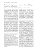
Figure 2 (top) plots the false discovery rate:
FDR = FP(q)/O
11
(q)
and false non-discovery rate:
FNR = FN(q)/(n - O
11
(q))
for 50 simulations carried out as described in Materials and
methods, for scenario I structure A. It is clear that R(q
max
) has
the smallest FDR. On the other hand, q
2

corresponds to the
intersection between FDR and FNR. Moreover, in Figure 2
(bottom) we show that the same threshold minimizes the glo-
bal misclassification error as the sum of false positives and
false negatives. Note that if we considered the minimum sig-
nificant ratio, defined as the minimum of the R(q) over the set
of credibility intervals excluding 1, FDR would increase dra-
matically and the FNR would decrease only marginally with
respect to R(q
max
) and R(q
2
). As expected, the global misclas-
sification error would also be much larger, making this rule
inappropriate.
When there are no ratios R(q) equal or greater than 2 (which
can happen in the case of large noise or when there is only a
small proportion of genes in common), this rule does not
apply and we recommend using the rule corresponding to
R(q
max
).
Our computations have been implemented in the statistical
programming language R [9]. The R package for simulating
the data, for the two tests and for visualizing the results is
called BGcom and is available on our project BGX website
[10].
Performance on simulated data
Besides assessing the operating characteristics of our pro-
posed rules, we also applied the method proposed by Hwang

et al. implemented in Matlab [11]. Note that their aim is to
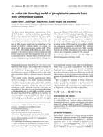
Typical plots of T(q) and R(q) for associated experiments (case A1)Figure 1
Typical plots of T(q) and R(q) for associated experiments (case A1). The two associated experiments were simulated under scenario I, structure A, with
true differences drawn from a Ga(2.5,0.4) and noise experiment specific of 0.5 and 0.8, respectively (signal-to-noise ratio = 9.6). The left plot shows the
distribution of T(q) and the right one shows the distribution of R(q) with Bayesian credibility intervals at 95%. T(q) shows a deviation from 1 for a p value
between 0.01 and 0.5. T(q
max
) is 2.6 and corresponds to a threshold q = 0.01. R(q) presents the same trend, but the estimates are slightly smaller since the
model takes into account the variability of the margins of the 2 × 2 table. The threshold associated with R(q) = 2 is 0.08. The number of genes in common
for each ratio R(q) is reported on the right axis of each plot.
P value
T
0 0.2 0.4 0.6 0.8 1
0
1
T
max
3,000
799
688
623
_
_
_
_
_
_
_
_
_

_
_
_
_
_
_
_
_
_
_
_
_
_
_
_
_
_
_
_
_
_
_
_
_
_
_
__
_
_
_

_
_
_
_
__
_
_
_
_
_
_
_
_
_
_
__
_
_
_
__
_
_
_
_
_
_
_
_
_
_

_
_
_
__
_
_
___
_
____
__
_
_
________
_
_
_
_
_
_
_
_
_
_
_
_
_
_
_
_
_

_
_
_
_
_
_
_
_
_
_
_
_
_
_
_
_
_
_
_
_
_
_
_
_
_
_
_
_
_
_

_
_
_
_
_
_
_
_
_
_
_
_
_
__
_
_
_
_
_
_
_
_
_
___
_
_
_
_
_
__

_
_
_
___
_
_
_
_
_
_
__
__
_
_
_
P value
R
0 0.2 0.4 0.6 0.8 1
0
1
R
2
R
max
3,000
799
688
623
2
R54.6 Genome Biology 2007, Volume 8, Issue 4, Article R54 Blangiardo and Richardson />Genome Biology 2007, 8:R54

integrate p values from different experiments in a meta-anal-
ysis and they present three statistics to do so: Fisher's
weighted F, Mudholkar-George's weighted T and Liptak-
Stouffer's weighted Z. We report Fisher's weighted F (the
default statistic in the Matlab function), defined as:
where w
k
is the weight for the k
th
experiment and p
gk
is the p
value for the gene g in the experiment k. F
g
will be a new glo-
bal p value that integrates those weights from different exper-
iments. The authors also present several rules to select
differentially expressed genes from F
g
, the simplest one using
a fixed threshold on the p values equal to 0.05, and others that
minimize the number of false positives and false negatives, in
a parametric or non-parametric framework. We follow the
authors' suggestion and use the non-parametric rule. For
more details on the method, see [2].
The behavior of T(q) and of the credibility intervals CI
95
(q) for
a typical simulation are displayed in Figure 1 (associated
experiments) and Figure 3 (independent experiments). When

the two experiments are not associated (the number of simu-
lated genes in common is equal to 0), the plot of T(q) for dif-
ferent cut-offs q is, as expected, a horizontal line of height 1,
with evidence of noise for small p values. In the same Figure,
one sees that all the credibility intervals derived by the Baye-
sian procedure include the value 1 and have decreasing width
as q gets larger, as expected.
In the case of two independent experiments we never declare
any gene to be in common in any of the 50 simulations, so our
procedure has no error. On the other hand, Hwang et al.'s
method picks up 320 genes on average (Table 3, independ-
ence case), which are all false positives.
When there is a positive association between the two experi-
ments, T(q) can assume two shapes: it can decrease monoton-
ically as the p values increase (Figure 1), or reach a peak and
then decrease (Additional data file 1) as the p values increase.
The Bayesian estimates exhibit a similar shape, but since in
this approach the variability of the denominator of T(q) is
modeled, the resulting ratio estimates are smoothed.
We see that our proposed method gives a sensible and inter-
pretable procedure, with a pattern that is easily distinguisha-
ble from that of the no association case. This is confirmed by
the results given in Table 4.
Scenario I mimics a realistic situation where the two experi-
ments have different degrees of differential expression and
consequently quite different list sizes at any given signifi-
cance level. It supposes that the list of genes is divided into
four groups: genes differentially expressed in both experi-
ments, genes differentially expressed in only one of the two
experiments, and genes differentially expressed in neither

experiment. The first group identifies the 'true positive genes'
that we want to detect by our method. The remaining groups
act like additional noise to make the set up more realistic. We
also define a different scenario (scenario II) to mimic a situa-
tion where the two experiments have similar size of differen-
tial expression. It only supposes the genes are divided into
two groups: differentially expressed genes in both experi-
ments and differentially expressed genes in no experiment.
We describe the simulation set up in detail in Materials and
methods.
Misclassification error, false discovery and false non-discovery rates for case A2 (results are averaged over 50 replicates)Figure 2
Misclassification error, false discovery and false non-discovery rates for
case A2 (results are averaged over 50 replicates). The upper plot shows
the false discovery rate (FDR) and the false non-discovery rate (FNR) for
case A2. The FDR is calculated as the ratio of the false positives to the
number of genes called in common, while the FDR is calculated as the
ratio of the false negatives to the number of genes not called in common.
The true differences d
g
are drawn from a Ga(2, 0.5) and the noise
component experiment specific is 2 for the first experiment and 3 for the
second. R(q
max
) shows the minimum FDR. On the other hand, R(q
min
) has
a very large FDR and the improvement of the FNR is slight. As a
compromise, the threshold q
2
is close to q

max
, so guarantees a low FDR,
but returns a larger list. It approximatively corresponds to the intersection
point between the two curves of FDR and FNR. The lower plot shows the
global error as the sum of FP and FN. The threshold associated with R(q
2
)
is very close to the minimum of the curve, that is, to the smallest global
misclassification error.
0.0
0.2
0.4
0.6
P value
q
max
q
2
0.2 0.3 0.4
q
min
0.6 0.7 0.8 0.9
1
FDR
FNR
500
1,000
1,500
2,000
P value

q
max
q
2
0.2 0.3 0.4
q
min
0.6 0.7 0.8 0.9
1
FP + FN
Fwp
gkgk
k
=−
=
∑
2
1
2
ln()
Genome Biology 2007, Volume 8, Issue 4, Article R54 Blangiardo and Richardson R54.7
comment reviews reports refereed researchdeposited research interactions information
Genome Biology 2007, 8:R54
In both scenarios, structure A refers to experiments where
there would be a large proportion of genes in common relative
to the total number of differentially expressed genes. Case A1
is characterized by a large true difference between conditions
and a small experiment-specific error, giving an average sig-
nal-to-noise ratio of 9.6. Our first rule returns a ratio T(q
max

)
= 2.61 that is associated with q
max
= 0.01. In this case the aver-
age number of genes in the common list associated with the
max ratio is O
11
(q
max
) = 619, while that expected is
and the permutation based test returns a
significant Monte Carlo p value ≤ 0.001. The Bayesian ratio
R(q
max
) is slightly smaller than T(q
max
); accounting for varia-
bility in the Bayesian model results in wide CIs for small p val-
ues as previously pointed out. Our methodology gives
excellent results in this case, with the sum of false positives
and false negatives equal to 89, while the FDR is 0.006 and
the FNR is 0.036. Moving from q
max
to q
2
, the number of
genes called in common by this procedure is 676, which is
very close to the true number of common genes set in the
simulation (700). The number of false positives is larger than
the one corresponding to q

max
, but still quite small, whilst the
number of false negatives decreases appreciably, so that the
global error reaches its minimum value (83). Note that both
q
max
and q
2
generate a far smaller global error than Hwang et
al.'s procedure (Table 3).
Moving to case A2, the noise associated with the experiment
increases and the true differences between conditions are
smaller. This results in fewer genes called in common and a
corresponding increase in the global error. Nevertheless, all
the cases present the same trend: q
max
is associated with the
synthesized list having the smallest number of false positives
and the list given by q
2
is close to the one with the smallest
global error. Moreover, for both cut-offs our methodology
consistently leads to smaller errors than that of Hwang.
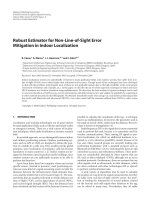
Typical plots of T(q) and R(q) in the case of independent experimentsFigure 3
Typical plots of T(q) and R(q) in the case of independent experiments. The two independent experiments are simulated under scenario I, structure A, with
true differences drawn from a Ga(1, 1) and noise experiment specific of 2 and 2.5, respectively (signal-to-noise ratio = 0.4). The left plot shows the
distribution of T(q) and the right one shows the distribution of R(q) with Bayesian credibility intervals at 95%. T(q) follows a horizontal line of height 1
(independence between the lists) and presents instability for small p values (left tail). The Bayesian model does not present any significant threshold for
which R(q) deviates from 1 and the CI
95

always includes 1.
P value
T
0 0.2 0.4 0.6 0.8 1
0
_
_
_
_
_
_
_
_
_
_
_
_
_
_
_
_
_
_
_
_
_
_
_
_
_

_
_
_
_
_
_
_
_
_
_
_
_
_
_
_
_
_
_
_
_
_
_
_
_
_
_
_
_
_
_

_
_
_
_
_
_
_
_
_
_
_
_
_
_
__
_
_
_
_
__
_
_
_
_
_
_
_
_
_
_

_
_
_
_
_
_
_
_
_
__
_
_
_
_
_
_
_
_
_
_
_
_
_
_
_
_
_
_
_
_

_
_
_
_
_
_
_
_
_
_
_
_
_
_
_
_
_
_
_
_
_
_
_
_
_
_
_
_
_
_

_
_
_
_
__
_
_
_
_
_
_
_
_
_
_
_
__
_
_
_
_
_
_
_
_
_
_
_
_
_

_
_
_
_
_
_
_
_
_
_
_
_
_
_
_
_
P value
R
0
0 0.2 0.4 0.6 0.8 1
11
975 730
3000
237
×
=
R54.8 Genome Biology 2007, Volume 8, Issue 4, Article R54 Blangiardo and Richardson />Genome Biology 2007, 8:R54
Simulations under structure B and C mimic cases where there
is a smaller proportion of genes in common relative to the
total number of differentially expressed genes. For cases B1

and C1 the noise is very small and the true difference between
conditions is large; cases B2 and C2 are characterized by a
smaller true difference and a higher noise. The pattern
remains the same in cases A1 and A2: the list associated with
q
max
shows the smallest number of false positives, while the
one associated with q
2
is very close to the minimum global
error. Again our rules show a far smaller global error that
those of Hwang. Note that for cases B1 and C1, there is no q
2
and q
max
is associated with the smallest global error. Addi-
tional simulations are presented in Tables 1 and 2 of Addi-
tional data file 1.
Scenario II shows a similar trend confirming that our method
also works well in a different experimental framework. We
still find very few false positives with both rules q
max
and q
2
.
On the other hand, the sensitivity is generally higher than in
scenario I for both rules, hence the global error is smaller.
This results in a better performance of the maximum q
max
: it

shows no false positive in all the cases of this scenario and
since the false negatives are generally fewer, its global error is
quite small and, in some cases, smaller than the one for q
2
.
Hwang et al.'s method shows an improvement in terms of
false positives with respect to scenario I, while the false nega-
tives remain quite the same. This is to be expected because, in
this scenario, the intersection and the union of differentially
expressed genes are identical. Nevertheless, our method also
performs better in most of the cases in this scenario, with the
exception of case A2, where our global error is 509 for the q
2
rule while Hwang et al.'s is 450. However, we still halve the
number of false positives. See Tables 3 and 4 of Additional
data file 1 for the results under scenario II.
Common features related to ventilation-induced lung
injury
We applied our methods to lists of p values for 2,769 mouse
and rat orthologs deriving from a study investigating the del-
eterious effects of mechanical ventilation on lung gene
expression through a model of mechanical ventilation-
induced lung injury (VILI; see Materials and methods for
details of this study). Results from the joint model are sum-
marized in Table 5 and the plots are presented in Figure 2 of
Additional data file 1. The conditional model returns nearly
identical results. Due to the large variability there is no
threshold associated with a R(q) ≥ 2, so we present the results
related to q
max

. The number of differentially expressed genes
common to both species is estimated as 97, which corre-
sponds to 63 orthologs (note that each probeset of one species
can be associated with several probesets of the other). These
are presented in Additional data file 1, which shows the
Table 3
Performance of Hwang et al.'s method on simulated data for scenario I
DE nonD
E
FP (%) TP (%) FN (%) TN (%) Global
error
Global error
R(q
2
)
Independent case: n = 3000, common = 0, DE1 = 1000, DE2 = 800 320 2,680 320
(10.7)
0 0 2,680
(89.3)
320 0
A: n = 3000, common = 700, DE1 = 1000, DE2 = 800
Case A1 1,121 1,879 440
(19.1)
681
(97.3)
19 (2.7) 1,860
(80.9)
459 82
Case A2 409 2,591 188 (8.2) 221
(31.6)

479
(68.4)
2,112
(91.8)
667 544
B: n = 3000, common = 200, DE1 = 700, DE2 = 500
Case B1 999 2,001 805
(28.8)
194
(97.0)
6 (3.0) 1,996
(71.2)
811 31*
Case B2 427 2,573 333
(11.9)
94 (47.0) 106
(53.0)
2,467
(88.1)
439 165
C: n = 3000, common = 100, DE1 = 500, DE2 = 400
Case C1 816 2,185 718
(24.8)
97 (97.1) 3 (2.9) 2,182
(75.2)
721 19*
Case C2 346 2,654 299
(10.3)
47 (47.0) 53 (53.0) 2,601
(89.7)

352 84
Average simulation results: we present the results from Hwang et al.'s method on the simulated data under scenario I. DE1 and DE2 are the
differentially expressed genes in the first and the second experiment respectively. We used the Fisher's weighted F defined as
, where w
k
is the weight for the k
th
experiment and p
gk
is the p value for the gene g in the experiment k. We present the
non-parametric rule to select the differentially expressed (DE) genes, as suggested by the authors. The method is implemented in Matlab. In the last
column we report the Global error (FP + FN) of our procedure for q
2
(see Table 2) for ease of comparison. *There is no ratio larger than 2 so the
maximum rule has been used in this case.
Fwp
gkgk
k
=−
=
∑
2
1
2
ln()
Genome Biology 2007, Volume 8, Issue 4, Article R54 Blangiardo and Richardson R54.9
comment reviews reports refereed researchdeposited research interactions information
Genome Biology 2007, 8:R54
number of ortholog pairs in common out of the number of
ortholog pairs measured.

We compared our results to those obtained applying Hwang
et al.'s method, also presented in Table 5. The latter picked
1,425 globally differentially expressed genes using the non-
parametric rule. The 97 genes in common found by our
method are included in their list, which is not surprising since
ours focuses on the intersection of the two lists of p values,
while theirs tests their union.
Table 4
Performance on simulated data for scenario I
Parameters Rules q R CI
95
O
11
O
1+
O
+1
FP (%) TP (%) FN (%) TN (%) Global error
Independence case: n = 3000, common
= 0, DE1 = 1000, DE2 = 800
Independence: signal to noise 0.55 1* 0.98-1.02 0
†
0
†
0
†
0 0 0 3,000 (100.0) 0
ratio = 0.4
‡
A: n = 3000, common = 700, DE1 =

1000, DE2 = 800
Case A1: signal to noise ratio = 9.6
‡
Max 0.01 2.60 2.50-2.72 619 975 730 4 (0.2) 615 (87.8) 85 (12.2) 2,296 (99.8) 89
Double 0.06 2.04 1.97-2.19 676 1,095 877 29 (1.3) 647 (92.4) 53 (7.6) 2,271 (98.7) 82
Min
§
= 81
Case A2: signal to noise ratio = 1.6
‡
Max 0.01 4.72 4.19-5.29 86 346 157 1 (0.0) 85 (12.1) 615 (87.9) 2,299 (100.0) 616
Double 0.08 2.01 1.90-2.20 212 677 459 28 (1.2) 184 (26.3) 516 (73.7) 2,272 (98.8) 544
Min
§
= 535
B: n = 3000, common = 200, DE1 = 700,
DE2 = 500
Case B1: signal to noise ratio = 9.6
‡
Max
¶
0.01 1.72 1.58-1.86 185 691 467 8 (0.3) 177 (88.5) 23 (11.5) 2,792 (99.7) 31
Min
§
= 31
Case B2: signal to noise ratio = 1.6
‡
Max 0.01 2.98 2.38-3.71 36 250 145 3 (0.1) 33 (16.7) 167 (83.3) 2,797 (99.9) 170
Double 0.03 2.03 1.67-2.40 57 355 236 11 (0.4) 46 (23.0) 154 (77.1) 2,789 (99.6) 165
Min

§
= 165
C: n = 3000, common = 100, DE1 = 500,
DE2 = 400
Case C1: signal to noise ratio = 9.6
‡
Max
¶
0.01 1.48 1.30-1.67 95 500 383 7 (0.2) 88 (88.4) 12 (11.6) 2,893 (99.8) 19
Min
§
= 19
Case C2: signal to noise ratio = 1.6
‡
Max 0.01 2.93 2.16-3.83 20 214 96 3 (0.1) 17 (16.6) 83 (83.4) 2,897 (99.9) 86
Double 0.02 2.16 1.63-2.81 26 262 134 5 (0.2) 21 (21.0) 79 (79.0) 2,895 (99.8) 84
Min
§
= 84
Average simulation results: we show the results from the joint model on one case of simulated data for independent experiments and six cases of simulated data for two
associated experiments. The simulation scenario consists of four groups of genes: differentially expressed DE in both experiments, differentially expressed in only one
experiment (DE1 and DE2 respectively), and differentially expressed in neither experiment. For the Independence case, the number of genes differentially expressed in both
experiments was set to 0. We present two decision rules: the threshold associated with the maximum R(q) is q
max
and the threshold associated with the R(q) ≥ 2 is q
2
(called
'double' in the table). We define q
max
= arg max{Median(R(q) | O, n) over the set of values of q for which CI

95
(q) excludes 1} and q
2
= max{over the set of values of q for which
CI
95
(q) excludes 1 and Median(R(q) | O, n) ≥ 2}. We averaged the results over 50 repeats for each case. *In case of independence it is still possible to calculate he maximum of
R(q), but it is not significant, so there is no associated list of common genes.
†
All the CIs contain 1, so no genes are called in common; thus, there are no FP.
‡
The signal to ratio
is calculated as E(Ga(shape, 1/scale))/(r
1
/2 + r
2
/2).
§
Minimum global error (observed).
¶
There is no ratio larger than 2 and only the maximum rule has been reported.
Table 5
Results from the VILI experiment
Joint Bayesian model Hwang et al.'s method
q
max
R(q
max
) O
11

O
1+
O
+1
CI
95
DE nonDE
0.01 1.43 97 393 886 1.13-1.75 1,425 3,734
The number of genes in common is 97, which corresponds to 63 orthologs. The conditional model shows the same results (not reported). The
procedure indicates clearly a significant association between the two lists. Hwang et al.'s method calls 1,425 genes as differentially expressed (DE). All
the genes reported by our method are included in their list.
R54.10 Genome Biology 2007, Volume 8, Issue 4, Article R54 Blangiardo and Richardson />Genome Biology 2007, 8:R54
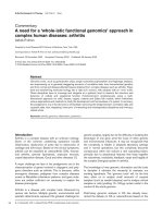
This difference is highlighted in Figure 4 (left), which plots
mice fold change versus rats fold change on the natural loga-
rithmic scale: it is apparent that genes highlighted by Hwang
et al.'s method but not by ours (+) have log fold change close
to 0 for one of the species, while the genes highlighted by both
the methodologies (o) present large fold changes for both the
species. The correlation between the fold changes measured
in the two experiments is 0.4 for the 97 orthologs returned by
our procedure and 0.06 for the other 1,328 genes picked up
only by Hwang et al.'s method, confirming how our method-
ology focuses attention on the genes differentially expressed
in both experiments.
We used fatiGO [12] to annotate the common set of orthologs
found by our analysis: 24 genes are involved in one or more
pathways described in the Kyoto Encyclopedia of Genes and
Genomes (KEGG), 42 are annotated at the third level of the
Gene Ontology (GO) as part of biological processes, 41 belong
to molecular functions and 36 to cellular components. See

Additional data file 2 for the complete list of GO categories
and KEGG pathways.
Out of the biological processes, the most represented are
related to the integrated function of a cell ('cellular
physiological process', 'metabolism', 'regulation of cellular
process', 'regulation of physiological process'), showing
between 38 and 15 orthologs in common. In addition, there
are some other interesting processes related to responses of
the body to stress and external or endogenous stimulus; these
can be related to the effect of mechanical ventilation, which
acts as an external stimulus and also causes stress on cells.
From the KEGG pathways, we focus attention on the two
most represented categories: the 'MAPK signaling activity'
and the 'Cytokine-cytokine receptor interaction'. Six of the
orthologs found to be significant are involved in the first
(Fgfr1, Gadd45a, Hspa8, Hspa1a, Il1b, Il1r
2
). The involve-
ment of this pathway is again suggestive of how mechanical
Log fold change (natural log) for the VILI experiment (left) and high-fat diet experiment (right)Figure 4
Log fold change (natural log) for the VILI experiment (left) and high-fat diet experiment (right). The left plot shows the log fold changes for mice versus rat
averaged over the two replicates for each species. The right plot shows the log fold changes for fat versus muscle averaged over the three and four
replicates for each species. The circles correspond to the genes highlighted by our analysis and by the method of Hwang et al.; they are characterized by a
large log fold change for both the species. The correlation of the two fold changes for this group is 0.4 (VILI experiment) and 0.8 (high-fat diet experiment).
The crosses correspond to the genes highlighted only by Hwang et al.'s analysis; they are characterized by a large log fold change for one species and a
small fold change for the other one. The correlation of the two fold changes for this group is 0.06 (VILI experiment) and 0.36 (high-fat diet experiment).
−2 −1 0 1 2
−2
−1
0

Mice log fold change
Rats log fold change
+
+
++
+
+
+
+
+
+
+++
+
++++++
+
+++
++
++
+
+
++
+++
+
+
+
+
+
+
++
++

+
++
++
+
+
+
+
+
+
+
+
+
+++
+
+
+
+
+
+
+
+
+
+
++
+
++
+
+
++
+

+
+
+
+
+
+
++
++
+
++
++
+++
+
+
+
+
+
+
+
+
++
+
+
+++
++
+
+
+
+
++

++
+
++
+
+
++
+
+
+++
+
+
+
+
+++
+
+
+
+
+
++
+
++
++
++
+
+
+
+
+
+

+++++
++
+
++++
+
+
+++
+++
+
++
+++++
+
+
+++
+
+
+
++
++
+
++
+
+
+
+
+
+
+
++
++

+
++
+
+
+
+
+
+
+
+
+
+
+
++
+
+
+
+
+
+
+
+
+
+
+
++
+
+
++
++

+
+
+
+
+
+++
+
+++
+
++
+
+
+
+
+
+
+
++
+
+
+
++
+
+++++
+
+
+
+
++
+

++
+
+
+
+
++
++
+
+
+
+
+
+
+
++
++
++
+
+
+
+
+
+
+
+
+
+
++
+
+

+
+++
+
+
+
+
+++
+
+
+
+
+
+
+
++
+
+
+
+
++
++
+
+
+++
+
+
+++
+
+
+

+++
++
++
++
++
++
+
+
+
+
++
+
+
++
++
+
+
++
+
++
+
+
+
+
++
+
+
+
+
+

+
+
++
+
++
+
+
+
+
+
+
++
++
+
+
+
+
+
+++
+
+
+
+
+
+
+
+
+
++
++

+
+
++
+
+
+
++
++
+
+
+
+++
+
+
+
+
++
++
+
+
++
+
++
+
+
++
+
++
+
+

+
+
+
+
+++
+
+++
++
+
++
++
+
+
+++
+
+
+
++
+
+
+
+
+++
+
+
+
++
+
+++
+

+
+
++
+
+++
+
+
+
+
+
+
+
+
+
+
+
++
++
+
+++++
+
+
+
+
+
+
+
+
+
+

+
+
+
+
+
+
+
+
+
+
+
+++
+
+
+
++
++
+
+
+
+
+
+
+
++
+
+
+
+
+

+
+
+
+
+
+
+
+
+
+
+
+
++
+
+++
+
+
++
+
+
+
+
+
++
+
+
+
+
+
+

+
+
+
+
+++
++
+
+
+
+
+
+
+
+
+
+
+
+
++
+
++
++
+
+
++
+
+
+
++
+

++
+
+
+
+
+
+
++
+
+
+
++
++
+
++
+
+
+++
+
+
+
+
+++
+
++
+
+
+
+
+

+
++
++
++
+
++
+
+
++
+
+
+
+
++
+
+
+
++
+
+
+
+
+
++
+
+
++
+
++
+

++
+
+
++
+
++
+
+
+
+
++
+
+
+
+
+
+
++
+
+
++
++
++
+
+
++
+
+++
+
+++

+
+
+
+
+
++
+
++
+
+++
+
+
+
+
+
++
+
+
+
+
+
+
+
++
++
+
+
+
+
+

+
+
++
+
+
+
+
++
+
+
+
+
+
+
+
+
++
+
+
+
++
+
+
+
+
++
+
+
+
+

+
+
+
+
++
++
+
++
+
+
+
++
+
+
++
+
+
++
++
+
+
++
++
+
++
+
+
++
++
+

++
++
+
+
++
+
+
+
+
+++
++
++
+
+
++
+
+
+
+
+
++
+++
+
+++
+
+
+
+
+
++

+
+
++
+
++
+
+
+
++
+
++
++
++
+
+
+
+
++
+
+
+
+++
+
+
+
+
+
+
+
+

+
+
+
+
+
+
++
+
++
+
+++
+
++
++
+
+
+
+
++
++
++
++
+
+
++
+
+
+
+
+

++
++
+
+++
++
+++
+
+++
++
+
+
+
+++
++
+
+
+
+
++
+
+
+
+
+
+++
+
+
+
+
+

+
+
+
+
+
++
++
+
+
+
+
++
+
+
+
+
+
+
++
++
+
+
+
+
++
++
+
+
++
++

+
++
+
+
+
+
++
+
+
++
+
++
+
+
++
+
++
+
+
+
+
+
+
+
+
+
++
+
+
+

++
+
+
++
+
+
+
++
+
+
++
+
+
+++
+
+
++
+
+
+
+
+
+
+
+
++
+
+
+
+

+
+
+
+
++
+
++
++
+
+
+
++
+
+
+
+
+
+
+
+
+
+
+
+
++
+
+
+
+
+

+
+
+
+
+
+
+
++
+
+
+
+
+
+
+
++
+
+
+
+
+
+
+
++++
+
++
+
+
+
+

+
+
+
+
+
+
+
+
+
++
++
+
+
++
+
+++
+
++
−4 −3 −2 −1 0 1 2 3
Fat log fold change
Muscle log fold change
+
+
+
+
+
+
+
+
+

+
+
+
+
+
+
+
+
+
+
+
+
+
+
+
+
+
+
+
+
+
+
+
+
+
+
+
+
+
+

+
+
+
+
+
+
+
+
+
+
+
+
+
+
+
+
+
+
+
+
+
+
+
+
+
+
+
+
+
+

+
+
+
+
+
+
+
+
+
+
+
+
+
+
+
+
+
+
+
+
+
+
+
+
+
+
+
+
+
+

+
+
+
+
+
+
+
+
+
+
+
+
+
+
+
+
+
+
+
+
+
+
+
+
+
+
+
+
+
+

+
+
+
+
+
+
+
+
+
+
+
+
+
+
+
+
+
+
+
+
+
+
+
+
+
+
+
+
+
+

+
+
+
+
+
+
+
+
+
+
+
+
+
+
+
+
+
+
+
+
+
+
+
+
+
+
+
+
+
+

+
+
+
+
+
+
+
+
+
+
+
+
+
+
+
+
+
+
+
+
+
+
+
+
+
+
+
+
+
+

+
+
+
+
+
+
+
+
+
+
+
+
+
+
+
+
+
+
+
+
+
+
+
+
+
+
+
+
+
+

+
+
+
+
+
+
+
+
+
+
+
+
+
+
+
+
+
+
+
+
+
+
+
+
+
+
+
+
+
+

+
+
+
+
+
+
+
+
+
+
+
+
+
+
+
+
+
+
+
+
+
+
+
+
+
+
+
+
+
+

+
+
+
+
+
+
+
+
+
+
+
+
+
+
+
+
+
+
+
+
+
+
+
+
+
+
+
+
+
+

+
+
+
+
+
+
+
+
+
+
+
+
+
+
+
+
+
+
+
+
+
+
+
+
+
+
+
+
+
+

+
+
+
+
+
+
+
+
+
+
+
+
+
+
+
+
+
+
+
+
+
+
+
+
+
+
+
+
+
+

+
+
+
+
+
+
+
+
+
+
+
+
+
+
+
+
+
+
+
+
+
+
+
+
+
+
+
+
+
+

+
+
+
+
+
+
+
+
+
+
+
+
+
+
+
+
+
+
+
+
+
+
+
+
+
+
+
+
+
+

+
+
+
+
+
+
+
+
+
+
+
+
+
+
+
+
+
+
+
+
+
+
+
+
+
+
+
+
+
+

+
+
+
+
+
+
+
+
+
+
+
+
+
+
+
+
+
+
+
+
+
+
+
+
+
+
+
+
+
+

+
+
+
+
+
+
+
+
+
+
+
+
+
+
+
+
+
+
+
+
+
+
+
+
+
+
+
+
+
+

+
+
+
+
+
+
+
+
+
+
+
+
+
+
+
+
+
+
+
+
+
+
+
+
+
+
+
+
+
+

+
+
+
+
+
+
+
+
+
+
+
+
+
+
+
+
+
+
+
+
+
+
+
+
+
+
+
+
+
+

+
+
+
+
+
+
+
+
+
+
+
+
+
+
+
+
+
+
+
+
+
+
+
+
+
+
+
+
+
+

+
+
+
+
+
+
+
+
+
+
+
+
+
+
+
+
+
+
+
+
+
+
+
+
+
+
+
+
+
+

+
+
+
+
+
+
+
+
+
+
+
+
+
+
+
+
+
+
+
+
+
+
+
+
+
+
+
+
+
+

+
+
+
+
+
+
+
+
+
+
+
+
+
+
+
+
+
+
+
+
+
+
+
+
+
+
+
+
+
+

+
+
+
+
+
+
+
+
+
+
+
+
+
+
+
+
+
+
+
+
+
+
+
+
+
+
+
+
+
+

+
+
+
+
+
+
+
+
+
+
+
+
+
+
+
+
+
+
+
+
+
+
+
+
+
+
+
+
+
+

+
+
+
+
+
+
+
+
+
+
+
+
+
+
+
+
+
+
+
+
+
+
+
+
+
+
+
+
+
+

+
+
+
+
+
+
+
+
+
+
+
+
+
+
+
+
+
+
+
+
+
+
+
+
+
+
+
+
+
+

+
+
+
+
+
+
+
+
+
+
+
+
+
+
+
+
+
+
+
+
+
+
+
+
+
+
+
+
+
+

+
+
+
+
+
+
+
+
+
+
+
+
+
+
+
+
+
+
+
+
+
+
+
+
+
+
+
+
+
+

+
+
+
+
+
+
+
+
+
+
+
+
+
+
+
+
+
+
+
+
+
+
+
+
+
+
+
+
+
+

+
+
+
+
+
+
+
+
+
+
+
+
+
+
+
+
+
+
+
+
+
+
+
+
+
+
+
+
+
+

+
+
+
+
+
+
+
+
+
+
+
+
+
+
+
+
+
+
+
+
+
+
+
+
+
+
+
+
+
+

+
+
+
+
+
+
+
+
+
+
+
+
+
+
+
+
+
+
+
+
+
+
+
+
+
+
+
+
+
+

+
+
+
+
+
+
+
+
+
+
+
+
+
+
+
+
+
+
+
+
+
+
+
+
+
+
+
+
+
+

+
+
+
+
+
+
+
+
+
+
+
+
+
+
+
+
+
+
+
+
+
+
+
+
+
+
+
+
+
+

+
+
+
+
+
+
+
+
+
+
+
+
+
+
+
+
+
+
+
+
+
+
+
+
+
+
+
+
+
+

+
+
+
+
+
+
+
+
+
+
+
+
+
+
+
+
+
+
+
+
+
+
+
+
+
+
+
+
+
+

+
+
+
+
+
+
+
+
+
+
+
+
+
+
+
+
+
+
+
+
+
+
+
+
+
+
+
+
+
+

+
+
+
+
+
+
+
+
+
+
+
+
+
+
+
+
+
+
+
+
+
+
+
+
+
+
+
+
+
+

+
+
+
+
+
+
+
+
+
+
+
+
+
+
+
+
+
+
+
+
+
+
+
+
+
+
+
+
+
+

+
+
+
+
+
+
+
+
+
+
+
+
+
+
+
+
+
+
+
+
+
+
+
+
+
+
+
+
+
+

+
+
+
+
+
+
+
+
+
+
+
+
+
+
+
+
+
+
+
+
+
+
+
+
+
+
+
+
+
+

+
+
+
+
+
+
+
+
+
+
+
+
+
+
+
+
+
+
+
+
+
+
+
+
+
+
+
+
+
+

+
+
+
+
+
+
+
+
+
+
+
+
+
+
+
+
+
+
+
+
+
+
+
+
+
+
+
+
+
+

+
+
+
+
+
+
+
+
+
+
+
+
+
+
+
+
+
+
+
+
+
+
+
+
+
+
+
+
+
+

+
+
+
+
+
+
+
+
+
+
+
+
+
+
+
+
+
+
+
+
+
+
+
+
+
+
+
+
+
+

+
+
+
+
+
+
+
+
+
+
+
+
+
+
+
+
+
+
+
+
+
+
+
+
+
+
+
+
+
+

+
+
+
+
+
+
+
+
+
+
+
+
+
+
+
+
+
+
+
+
+
+
+
+
+
+
+
+
+
+

+
+
+
+
+
+
+
+
+
+
+
+
+
+
+
+
+
+
+
+
+
+
+
+
+
+
+
+
+
+

+
+
+
+
+
+
+
+
+
+
+
+
+
+
+
+
+
+
+
+
+
+
+
+
+
+
+
+
+
+

+
+
+
+
+
+
+
+
+
+
+
+
+
+
+
+
+
+
+
+
+
+
+
+
+
+
+
+
+
+

+
+
+
+
+
+
+
+
+
+
+
+
+
+
+
+
+
+
+
+
+
+
+
+
+
+
+
+
+
+

+
+
+
+
+
+
+
+
+
+
+
+
+
+
+
+
+
+
+
+
+
+
+
+
+
+
+
+
+
+

+
+
+
+
+
+
+
+
+
+
+
+
+
+
+
+
+
+
+
+
+
+
+
+
+
+
+
+
+
+

+
+
+
+
+
+
+
+
+
+
+
+
+
+
+
+
+
+
+
+
+
+
+
+
+
+
+
+
+
+

+
+
+
+
+
+
+
+
+
+
+
+
+
+
+
+
+
+
+
+
+
+
+
+
+
+
+
+
+
+

+
+
+
+
+
+
+
+
+
+
+
+
+
+
+
+
+
+
+
+
+
+
+
+
+
+
+
+
+
+

+
+
+
+
+
+
+
+
+
+
+
+
+
+
+
+
+
+
+
+
+
+
+
+
+
+
+
+
+
+

+
+
+
+
+
+
+
+
+
+
+
+
+
+
+
+
+
+
+
+
+
+
+
+
+
+
+
+
+
+

+
+
+
+
+
+
+
+
+
+
+
+
+
+
+
+
+
+
+
+
+
+
+
+
+
+
+
+
+
+

+
+
+
+
+
+
+
+
+
+
+
+
+
+
+
+
+
+
+
+
+
+
+
+
+
+
+
+
+
+

+
+
+
+
+
+
+
+
+
+
+
+
+
+
+
+
+
+
+
+
+
+
+
+
+
+
+
+
+
+

+
+
+
+
+
+
+
+
+
+
+
+
+
+
+
+
+
+
+
+
+
+
+
+
+
+
+
+
+
+

+
+
+
+
+
+
+
+
+
+
+
+
+
+
+
+
+
+
+
+
+
+
+
+
+
+
+
+
+
+

+
+
+
+
+
+
+
+
+
+
+
+
+
+
+
+
+
+
+
+
+
+
+
+
+
+
+
+
+
+

+
+
+
+
+
+
+
+
+
+
+
+
+
+
+
+
+
+
+
+
+
+
+
+
+
+
+
+
+
+

+
+
+
+
+
+
+
+
+
+
+
+
+
+
+
+
+
+
+
+
+
+
+
+
+
+
+
+
+
+

+
+
+
+
+
+
+
+
+
+
+
+
+
+
+
+
+
+
+
+
+
+
+
+
+
+
+
+
+
+

+
+
+
+
+
+
+
+
+
+
+
+
+
+
+
+
+
+
+
+
+
+
+
+
+
+
+
+
+
+

+
+
+
+
+
+
+
+
+
+
+
+
+
+
+
+
+
+
+
+
+
+
+
+
+
+
+
+
+
+

+
+
+
+
+
+
+
+
+
+
+
+
+
+
+
+
+
+
+
+
+
+
+
+
+
+
+
+
+
+

+
+
+
+
+
+
+
+
+
+
+
+
+
+
+
+
+
+
+
+
+
+
+
+
+
+
+
+
+
+

+
+
+
+
+
+
+
+
+
+
+
+
+
+
+
+
+
+
+
+
+
+
+
+
+
+
+
+
+
+

+
+
+
+
+
+
+
+
+
+
+
+
+
+
+
+
+
+
+
+
+
+
+
+
+
+
+
+
+
+

+
+
+
+
+
+
+
+
+
+
+
+
+
+
+
+
+
+
+
+
+
+
+
+
+
+
+
+
+
+

+
+
+
+
+
+
+
+
+
+
+
+
+
+
+
+
+
+
+
+
+
+
+
+
+
+
+
+
+
+

+
+
+
+
+
+
+
+
+
+
+
+
+
+
+
+
+
+
+
+
+
+
+
+
+
+
+
+
+
+

+
+
+
+
+
+
+
+
+
+
+
+
+
+
+
+
+
+
+
+
+
+
+
+
+
+
+
+
+
+

+
+
+
+
+
+
+
+
+
+
+
+
+
+
+
+
+
+
+
+
+
+
+
+
+
+
+
+
+
+

+
+
+
+
+
+
+
+
+
+
+
+
+
+
+
+
+
+
+
+
+
+
+
+
+
+
+
+
+
+

+
+
+
+
+
+
+
+
+
+
+
+
+
+
+
+
+
+
+
+
+
+
+
+
+
+
+
+
+
+

+
+
+
+
+
+
+
+
+
+
+
+
+
+
+
+
+
+
+
+
+
+
+
+
+
+
+
+
+
+

+
+
+
+
+
+
+
+
+
+
+
+
+
+
+
+
+
+
+
+
+
+
+
+
+
+
+
+
+
+

+
+
+
+
+
+
+
+
+
+
+
+
+
+
+
+
+
+
+
+
+
+
+
+
+
+
+
+
+
+

+
+
+
+
+
+
+
+
+
+
+
+
+
+
+
+
+
+
+
+
+
+
+
+
+
+
+
+
+
+

+
+
+
+
+
+
+
+
+
+
+
+
+
+
+
+
+
+
+
+
+
+
+
+
+
+
+
+
+
+

+
+
+
+
+
+
+
+
+
+
+
+
+
+
+
+
+
+
+
+
+
+
+
+
+
+
+
+
+
+

+
+
+
+
+
+
+
+
+
+
+
+
+
+
+
+
+
+
+
+
+
+
+
+
+
+
+
+
+
+

+
+
+
+
+
+
+
+
+
+
+
+
+
+
+
+
+
+
+
+
+
+
+
+
+
+
+
+
+
+

+
+
+
+
+
+
+
+
+
+
+
+
+
+
+
+
+
+
+
+
+
+
+
+
+
+
+
+
+
+

+
+
+
+
+
+
+
+
+
+
+
+
+
+
+
+
+
+
+
+
+
+
+
+
+
+
+
+
+
+

+
+
+
+
+
+
+
+
+
+
+
+
+
+
+
+
+
+
+
+
+
+
+
+
+
+
+
+
+
+

+
+
+
+
+
+
+
+
+
+
+
+
+
+
+
+
+
+
+
+
+
+
+
+
+
+
+
+
+
+

+
+
+
+
+
+
+
+
+
+
+
+
+
+
+
+
+
+
+
+
+
+
+
+
+
+
+
+
+
+

+
+
+
+
+
+
+
+
+
+
+
+
+
+
+
+
+
+
+
+
+
+
+
+
+
+
+
+
+
+

+
+
+
+
+
+
+
+
+
+
+
+
+
+
+
+
+
+
+
+
+
+
+
+
+
+
+
+
+
+

+
+
+
+
+
+
+
+
+
+
+
+
+
+
+
+
+
+
+
+
+
+
+
+
+
+
+
+
+
+

+
+
+
+
+
+
+
+
+
+
+
+
+
+
+
+
+
+
+
+
+
+
+
+
+
+
+
+
+
+

+
+
+
+
+
+
+
+
+
+
+
+
+
+
+
+
+
+
+
+
+
+
+
+
+
+
+
+
+
+

+
+
+
+
+
+
+
+
+
+
+
+
+
+
+
+
+
+
+
+
+
+
+
+
+
+
+
+
+
+

+
+
+
+
+
+
+
+
+
+
+
+
+
+
+
+
+
+
+
+
+
+
+
+
+
+
+
+
+
+

+
+
+
+
+
+
+
+
+
+
+
+
+
+
+
+
+
+
+
+
+
+
+
+
+
+
+
+
+
+

+
+
+
+
+
+
+
+
+
+
+
+
+
+
+
+
+
+
+
+
+
+
+
+
+
+
+
+
+
+

+
+
+
+
+
+
+
+
+
+
+
+
+
+
+
+
+
+
+
+
+
+
+
+
+
+
+
+
+
+

+
+
+
+
+
+
+
+
+
+
+
+
+
+
+
+
+
+
+
+
+
+
+
+
+
+
+
+
+
+

+
+
+
+
+
+
+
+
+
+
+
+
+
+
+
+
+
+
+
+
+
+
+
+
+
+
+
+
+
+

+
+
+
+
+
+
+
+
+
+
+
+
+
+
+
+
+
+
+
+
+
+
+
+
+
+
+
+
+
+

+
+
+
+
+
+
+
+
+
+
+
+
+
+
+
+
+
+
+
+
+
+
+
+
+
+
+
+
+
+

+
+
+
+
+
+
+
+
+
+
+
+
+
+
+
+
+
+
+
+
+
+
+
+
+
+
+
+
+
+

+
+
+
+
+
+
+
+
+
+
+
+
+
+
+
+
+
+
+
+
+
+
+
+
+
+
+
+
+
+

+
+
+
+
+
+
+
+
+
+
+
+
+
+
+
+
+
+
+
+
+
+
+
+
+
+
+
+
+
+

+
+
+
+
+
+
+
+
+
+
+
+
+
+
+
+
+
+
+
+
+
+
+
+
+
+
+
+
+
+

+
+
+
+
+
+
+
+
+
+
+
+
+
+
+
+
+
+
+
+
+
+
+
+
+
+
+
+
+
+

+
+
+
+
+
+
+
+
+
+
+
+
+
+
+
+
+
+
+
+
+
+
+
+
+
+
+
+
+
+

+
+
+
+
+
+
+
+
+
+
+
+
+
+
+
+
+
+
+
+
+
+
+
+
+
+
+
+
+
+

+
+
+
+
+
+
+
+
+
+
+
+
+
+
+
+
+
+
+
+
+
+
+
+
+
+
+
+
+
+

1
2
3
−2
−1
0
1
2
Genome Biology 2007, Volume 8, Issue 4, Article R54 Blangiardo and Richardson R54.11
comment reviews reports refereed researchdeposited research interactions information
Genome Biology 2007, 8:R54
ventilation acts as an external stimulus, causing
inflammation and eventually also apoptosis. The gene encod-
ing fibroblast growth factor receptor 1 (Fgfr1) seems particu-
larly interesting; it belongs to the GO category 'GO:0030324',
related to lung development.
Five of the orthologs found to be significant by our methodol-
ogy belong to the 'Cytokine-cytokine receptor interaction' cat-
egory (IL6, Il1b, Il1r
2
, Ccl2, Kit). This again suggests an
involvement of immune response in VILI for both species.
These results clearly show that our procedure gives a coherent
list of genes that are differentially expressed in both species
and is consequently a powerful procedure for finding com-
mon pathways of interest.
Common features related to high-fat diet
We applied our methodology to the list of 12,488 genes from
original experiments evaluating the effects of high fat diet
versus normal fat diet in muscle and adipose tissue of two

strains of mice (see Materials and methods for details of this
study). The results from the Bayesian model are reported in
Table 6 and Figure 5 and are confirmed by the conditional
model (data not shown). We include in the table both the
decision rules, q
max
and q
2
. The ratio R(q
max
) associated with
the first decision rule is 3.84 with a CI
95
of 3.17-4.44. The
number of genes in common is 49. On the other hand, the
ratio associated with the other decision rule, R(q
2
) is 2.04 and
it returns a CI
95
of 1.90-2.21. In this case the number of com-
mon genes is 226.
As was already ascertained with the VILI datasets, the list of
genes in common found using our methodology is contained
in that found using Hwang et al.'s methodology. The latter
declared 3,746 genes as differentially expressed (DE; Table 6)
and, looking at the fold changes of this (Figure 4, right), con-
firms again how our methodology finds the intersection
between experiments, while that of Hwang et al. tests their
union. The correlation of the two lists of fold changes for the

genes declared by our methodology and Hwang et al.'s is 0.8,
while that for the genes called only by Hwang et al.'s proce-
dure is 0.36. A union of differentially expressed genes from
muscle and fat inevitably contains many tissue-specific
responses, whereas the intersection has the potential to
reveal common underlying tissue adaptation or systemic
responses to a high fat diet switch.
The size of the differentially expressed genes for each cut-off
q is quite different for the two tissues. This is an example of
the simulated scenario I, where we clearly also expect to have
genes differentially expressed only in one tissue. For this rea-
son, we focused particular attention on the rule q
2
, which
showed a smaller global error under scenario I. Again, we
used fatiGO [12] to annotate the 226 genes found by the q
2
rule: 128 are involved in the GO category 'Biological proc-
esses', 107 in 'Molecular function' and 116 in 'Cellular compo-
nents'; 42 belong to at least one KEGG pathway. The complete
annotation is reported in Additional data file 3.
Of special note in the KEGG pathways are several classes of
genes involved in inflammation and glucose metabolism. It is
well known that insulin resistance in mammals is associated
Results from the high-fat diet experimentFigure 5
Results from the high-fat diet experiment. The left plot shows the distribution of T(q) and the center one shows the distribution of R(q) with Bayesian
credibility intervals at 95%. q
max
for the conditional model is 0.01 and returns 20 genes in the common list, whilst for the joint model it is 0.02 and returns
49 common genes. On the other hand, q

2
= 0.07 and the number of genes in common is 226. The left plot is a blow-up of the Bayesian model results, to
better visualize the trend for p values between 0 and 0.2. The number of genes in common for each ratio is reported on the right axis of each plot.
P value
T
0 0.2 0.4 0.6 0.8 1
0
1
3
T
max
4.6
_
_
_
_
_
_
_
_
_
_
_
_
_
_
_
_
_
_

_
_
_
_
_
_
_
_
_
_
_
_
_
_
_
_
_
_
_
_
_
_
_
_
_
_
_
_
_
_

_
_
_
_
_
_
_
_
_
_
_
_
_
_
_
_
_
_
_
_
_
_
_
_
_
_
_
_
_
_

_
_
_
_
_
__
_
__
__
_
__
__
__
_
__
_
_
_
_
_
_
_
_
_
_
_
_
_
_
_

_
_
_
_
_
_
_
_
_
_
_
_
_
_
_
_
_
_
_
_
_
_
_
_
_
_
_
_
_
_

_
_
_
_
_
_
_
_
_
_
_
_
__
_
_
_
_
_
_
_
_
_
_
_
_
_
_
_
_
_

_
_
_
_
_
_
__
_
_
_
_
_
_
_
_
_
_
_
_
_
_
__
P value
R
0 0.2 0.4 0.6 0.8 1
0
1
R
2
3

R
max
4.6
12,488
226
75
49
_
_
_
_
_
_
_
_
_
_
_
_
_
_
_
_
_
_
_
_
_
_
_

_
_
_
_
_
_
_
_
_
_
_
_
_
_
_
_
_
P value
R
0
1
R
2
3
R
max
4.6
0.05 0.1 0.15 0.2
12,488
226

75
49
2
R54.12 Genome Biology 2007, Volume 8, Issue 4, Article R54 Blangiardo and Richardson />Genome Biology 2007, 8:R54
with chronic inflammation in adipose tissue [13]. Indeed, the
top KEGG category in our analysis is 'Cytokine-cytokine
receptor interaction', and includes the genes Ccl2 and
Tnfrsf1b. The Ccl2 gene encodes a C-X-C family cytokine that
is a ligand for the receptor Ccr2, a key mediator of diet-
induced obesity and insulin resistance [14]. Tnfrsf1b encodes
a receptor for tumor necrosis factor, an inflammatory
cytokine that is well established to be an inducer of insulin
resistance in adipose tissue [15,16]. It is particularly interest-
ing, therefore, to see that inflammatory genes are also
perturbed in muscle by the switch to a high-fat diet, suggest-
ing that similar molecular events are brought about in these
two tissues in response to the change in diet. Another inter-
esting category at the top of the list is 'Neuroactive ligand
receptor interaction', which includes Leptin, GHR and
NR3C1. Leptin and growth hormone receptor (GHR) are
known in the literature to be associated with obesity and a
high-fat diet in several tissues [17]; nuclear receptor sub-
family 3, group C, member 1 (NR3C1) is a ligand-activated
transcription factor that interacts with high affinity with cor-
tisol and other glucocorticoids. It is involved in response to
stress and in the suppression of the immune system.
Activation of expression of NR3C1 within the liver may con-
tribute to the development of type 2 diabetes in mice [18] and
it has a role in liver glucose metabolism during fasting and in
diabetic mice [19]. It would be very interesting to further

investigate if its role is maintained in other tissues besides fat
and muscle, as suggested by our analysis.
The proposed method highlights some interesting GO catego-
ries as 'Mitochondrial function' (Cellular component: Mito-
chondrion) and 'Oxidative reactions' (Molecular functions
category) are highlighted. Oxidative stress in adipose tissue
and adipocytes is associated with the development of insulin
resistance [16,20], although the mechanisms underlying this
are not understood. Furthermore, there is impaired insulin-
stimulated mitochondrial energy production in muscle of
type 2 diabetic patients [21].
That these processes are identified using our method of ana-
lyzing differentially expressed genes from diet-induced obes-
ity shows the strength of our approach. Using a concise, well
calibrated list, features of known biological interest as well as
novel aspects (for example, the KEGG pathway 'Neuroactive
ligand-receptor interactions' and particularly the gene
NR3C1) can be identified for further investigation.
Modeling three way contingency tables
The methodology presented can be generalized to more than
two experiments. Suppose we want to compare m experi-
ments through m lists of p values. The associated contingency
table will have dimension 2
m
.
In an m-way table, different hypotheses of independence can
be considered [22]. We refer here to mutual independence as
a direct extension of what we presented for a 2 × 2 table and
discuss other types of independence in the Discussion.
Considering three experiments and using a similar notation

to that previously introduced, for each threshold q we define
the experiments mutually independent if:
The statistic T(q) is generalized to:
where O
1++
, O
+1+
, O
++1
are again the marginal number of dif-
ferentially expressed genes in each of the three experiments.
It is known from the literature [23] that each cell of a contin-
gency table conditional on the strata margins follows a hyper-
geometric distribution. Hence:
O
111
(q) ~ Hyper(O
1++
(
θ
), O
+11
(
θ
),
ν
).
and, as previously pointed out, T(q) is proportional to a
hypergeometric. Thus, the permutation based test can be
used again to evaluate the significance of T(q

max
).
Releasing the conditioning on the margins, the sampling
schema is multinomial, as presented in equation 3, but with
Table 6
Results from high-fat diet experiment
Joint Bayesian model Hwang et al.'s method
Rules qR(q) O
11
O
1+
O
+1
CI
95
DE nonDE
Max 0.02 3.83 49 1,893 85 2.72-4.68 3,746 8,742
Double 0.07 2.04 226 3,059 452 1.90-2.21 3,746 8,742
The joint model returns R(q
max
) = 3.83 with an associated credibility interval [3.17-4.44]. The conditional model shows the same results (data not
reported). The R(q
2
) is 2.04 and the CI is 1.90-2.21. The procedure indicates clearly a significant association between the two lists. Hwang et al.'s
method calls 3,746 genes as differentially expressed (DE). All the genes called by our method are included in their list.
Oq
O
n
111
111

2
()=
′′
++ + + ++
OO
Tq
Oq
OqOqOq
n
()
()
() () ()
=
××
++ + + ++
111
111
2
Genome Biology 2007, Volume 8, Issue 4, Article R54 Blangiardo and Richardson R54.13
comment reviews reports refereed researchdeposited research interactions information
Genome Biology 2007, 8:R54
2
m
- 1 parameters and the statistic of interest is a direct
extension of equation 4. The decision rules defined in equa-
tions 6 and 7 can be applied to R(q).
To show that this extended procedure works well for synthe-
sizing three lists of p values, we enlarged our simulations to
include a case of three experiments following scenarios I, B
and C already presented for two experiments.

Performing 50 simulations for each scenario, we found con-
sistent results. q
max
picks few genes and it is very conserva-
tive. It declares no false positives but, as expected, many false
negatives. On the other hand, q
2
shows a larger list than q
max
,
but is characterized by still few false positives and a global
error close to the minimum observed (see Table 5 of Addi-
tional data file 1 for the results).
Discussion
Intersecting lists of differentially expressed features is a nat-
ural way to synthesize experiments, but calls for a statistical
procedure to choose the cut-off on the ranked lists that is best
for balancing specificity and sensitivity.
We have demonstrated how our methodology gives statisti-
cally meaningful cut-offs and how it has the benefit of not
requiring the original data, but only a probability measure of
differential expression for each list, as a p value. For this rea-
son, it can easily be applied to many types of experiments,
including those carried out on different platforms or on dif-
ferent species. Moreover, the comparison can be performed at
the gene level or at the function level and uses the type of
classification function that is most relevant. In the latter case,
p values have to be related to each function instead of each
gene, using for instance the methodology for global testing of
biological functions described in Goeman et al. [24].

The list of p values is not the only possible strategy for ranking
the genes; on a probability scale, posterior probability for a
gene to be differentially expressed can also be used [25],
being aware that, in this case, the ranking should be inverted
so that large posterior probabilities correspond to genes most
differentially expressed. Outside the probability scale, the
fold change could also be used as a ranking variable. How-
ever, while the range based on the probability scale is easily
defined, that of the fold change will vary for each experiment
and researchers should define a global range of values that is
sensible for synthesizing all the comparisons.
We have simulated two scenarios that reflect different exper-
imental setups. Scenario I supposes that in the two experi-
mental conditions under study, there are some condition
specific genes, differentially expressed only in one of the two
experiments, as well as common genes. On the other hand,
scenario II supposes that all the genes are either differentially
expressed in both experiments or differentially expressed in
neither. Both scenarios are plausible, but we think that the
first one is more likely to occur when analyzing experimental
data. Indeed, in both our case studies, there was a strong indi-
cation towards scenario I, with different sized lists for each
species or each tissue (see in Tables 5 and 6 the differences
between O
1+
(q) and O
+1
(q)). It is thus particularly interesting
to focus attention on the common genes, because it returns
the ones conserved between species (VILI experiment) or

potentially responsible for some biological mechanisms that
remain the same between different tissues (high-fat diet
experiment).
Both the conditional and joint models we propose are based
on the simplifying assumption of independence within the set
of genes under study. This assumption allows one to define
the underlying distribution as multinomial, but is clearly an
oversimplification in the context of genomic data. We evalu-
ated through an additional set of simulations described in
Materials and methods how the results of our procedures
would be affected if the features in each experiment were cor-
related. We found that analyzing a correlated set of genes with
our method tends to inflate the estimates of the ratio under
both the conditional and joint models for small p values.
Hence, the threshold q
2
is larger than that for the simulation
of an independent set of genes (0.04 versus 0.02). Neverthe-
less, in terms of false positives, false negatives and global mis-
classification error, we find that performance is similar to
Table 7
Simulation schema
Common genes (DE in both experiments) DE only in first experiment DE only in second experiment Non DE
A 700 300 100 1,900
B 200 500 300 2,000
C 100 400 300 2,200
DE, differentially expressed.
R54.14 Genome Biology 2007, Volume 8, Issue 4, Article R54 Blangiardo and Richardson />Genome Biology 2007, 8:R54
when the genes are not correlated (see Table 6 and Figure 3 of
Additional data file 1).

These results show that even though the independence
assumption is unrealistic, it does not substantially alter the
performance of our method. To reduce the dependence, a
possible extension of our method would be to consider groups
of differentially expressed features that are linked through
common pathways, for example, and to test whether the same
groups are commonly perturbed across different
experiments.
In the previous section, we also showed how we can extend
our method to more than two experiments, focusing attention
on three lists, but we stress that our methodology is readily
extendable to more than three experiments. Since the mar-
ginal distribution of a multi-hypergeometric is again hyperge-
ometric, the calculations are simplified and the computing
time does not increase exponentially from the two lists com-
parison case. Another convenient feature of our framework is
that it can be applied to evaluate a variety of independence
models for more than two experiments. We focused attention
on mutual independence, but hypotheses of conditional inde-
pendence or joint independence [22] can also be considered.
The definitions of T(q) and R(q) have to be modified accord-
ingly, but the methodology can be applied as it is. Moreover,
the interest can be focused on negative association as well,
which is on the O
1+
(q) - O
11
(q) and O
+1
(q) - O

11
(q) cells in the
2 × 2 table, corresponding to clearly specific features in each
experiment that are not found under the other conditions.
We have presented two alternative rules to select the list of
interest: the first is associated with the maximum ratio R(q),
which quantifies the largest deviation from the independ-
ence. It is very specific but rather conservative and tends to
select small lists. To achieve larger and balanced lists we have
proposed a second rule based on a ratio R(q) ≥ 2 and have
shown that this leads to the smallest observed global misclas-
sification error (FP + FN). The comparison to Hwang et al.'s
method has pointed out that our two rules perform better in
terms of global error in a variety of realistic simulated scenar-
ios. As a general comment, we suggest that the pattern of R(q)
ratios and associated significant credibility intervals are also
discussed with the experimentalists, who can select between
q
max
and q
2
for the threshold most appropriate to their exper-
imental context in terms of the relative weights of specificity
and sensitivity.
Conclusion
We have presented a simple methodology to synthesize sev-
eral experiments with the aim of finding a statistically mean-
ingful list of features that are perturbed in both (all)
experiments and demonstrate that our procedures have
excellent specificity and good sensitivity. They are applicable

to a wide range of experiments and comparisons. They pro-
vide experimentalists with powerful exploratory tools that
can help select a list of features of interest for further biologi-
cal investigation, as demonstrated by our analysis of two real
experimental datasets.
Materials and methods
Simulated data
To assess the performance of our methodology we use batches
of simulation. We follow the simulation set up described in
[2], so that comparison between the two approaches is easier.
Considering two experiments (k = 1,2), each of them with two
conditions, and n genes, for each gene we simulate a true dif-
ference between the conditions δ
g
, drawn from a gamma dis-
tribution with random sign. The true difference δ
g
is 0 if the
gene is not differentially expressed. We then add a normal
random noise, r
k
ε
gk
, where r
k
is the experiment specific com-
ponent and
ε
gk
is drawn from a standard Gaussian

distribution and is experiment and gene specific. We set up
two scenarios. In the first, which we call scenario I, we divided
the n genes into four groups: genes differentially expressed in
both experiments, genes differentially expressed only in the
first experiment, genes differentially expressed only in the
second experiment and genes differentially expressed in nei-
ther experiment. In the second scenario, called scenario II, we
divided the genes into only two groups: genes differentially
expressed in both experiments and genes differentially
expressed in neither experiment. Scenario II is thus a partic-
ular case of scenario I, which assumes strong communality
between the two experiments. When the genes are differen-
tially expressed in both experiments, they share the same δ
g
and the only difference between them is given by the random
components:
T
g1
=
δ
g
+ r
1
·
ε
g1
T
g2
=
δ

g
+ r
2
·
ε
g2
where T stands for the fold change on the logarithmic scale.
This group represents the 'true positive genes' (that is, truly
differentially expressed in both experiments) that we are
interested in finding using our method. In scenario I, the two
groups of genes differentially expressed only in one of the two
experiments act like additional noise and make the simula-
tion more biologically realistic. Together with the genes not
differentially expressed they constitute the 'negative genes' in
this setup, that is, genes that should not be listed if the proce-
dure correctly identifies the intersection.
Then, as described in [2], a two tailed t-test is performed for
each T
gk
and a p value is generated as:
pN
T
r
gk cdf
gk
k
=−
⎛
⎝
⎜

⎜
⎞
⎠
⎟
⎟
2||
Genome Biology 2007, Volume 8, Issue 4, Article R54 Blangiardo and Richardson R54.15
comment reviews reports refereed researchdeposited research interactions information
Genome Biology 2007, 8:R54
Both our method and that of Hwang et al. use the lists of p val-
ues as a starting point, so we implemented both procedures
and compared the results in terms of false positives and false
negatives. To be precise, we call a gene a false positive (FP) if
it is not differentially expressed in both the experiments but
is called in common by the methodology, and we call a gene a
false negative (FN) if it is differentially expressed in both the
experiments but is not declared as in common by the method-
ology. We also report the complementary quantities of true
positives (TP) and true negatives (TN) that characterize the
sensitivity and the specificity, respectively, of a rule. For each
scenario, we defined three structures, differing in the size of
intersection (Table 7).
Within each structure we further varied the value of the true
differences and the level of noise for each experiment, giving
cases 1 and 2. In case 1, the true differences δ
g
are drawn from
a Ga(2.5,0.4) and the level of noise is very small (r
1
= 0.5 and

r
2
= 0.8). In case 2, the true differences δ
g
are drawn from a
Ga(2,0.5) and the level of noise is larger (r
1
= 2 and r
2
= 3). We
also simulated a null scenario where the experiments are
independent and do not share values of δ
g
, with 1,000 genes
differentially expressed only in the first experiment, 800 dif-
ferentially expressed only in the second and 1,200 not differ-
entially expressed. For scenario II we replicated the same
structure and cases but with only two groups of genes. For
every case, we performed 50 simulations and averaged the
results for both the methods. Additional simulation results
with different levels of differential expression and noise can
be found in Tables 1 and 2 of Additional data file 1.
Simulated data for three lists
We simulated data from three experiments adapting case 2 of
scenario I, structures B and C. The true differences δ
g
are
drawn from a Ga(2,0.5) and the experiment specific noises
are r
1

= 2, r
2
= 2.5, r
3
= 3. For structure B, we considered 200
genes in common, out of 700 differentially expressed in the
first experiment, 600 differentially expressed in the second
experiment and 500 differentially expressed in the third
experiment. For structure C, we set 100 genes in common, out
of 500 differentially expressed in the first experiment, 400
differentially expressed in the second experiment and 300
differentially expressed in the third experiment.
Simulated data for a correlated set of genes
We simulated log gene expression data for 3,000 genes for
two experiments with two classes. For each experiment the
log gene expressions were drawn from a multivariate normal
distribution and we imposed a correlation matrix adapted
from experimental data we have been analyzing (BAIR
project [26]). For the first experiment, the quartiles of the
correlation coefficients are -0.86, -0.22, 0.01, 0.25, 0.85,
while for the second experiment they are -0.96, -0.27, 0, 0.28,
0.97. The mean variance for the first experiment is 1.32 and
for the second is 0.80. We divided the 3,000 genes into four
groups following the setup described before in accordance
with scenario I, structure A. For the differentially expressed
genes the log expression of the first class was drawn from a
multivariate normal with mean 12, while the log expression of
the other class was drawn from a multivariate normal with
mean equal to 5; for the not differentially expressed genes
both the log expressions were drawn from a multivariate nor-

mal with mean 5. Out of the 3,000 simulated genes, the 700
in 'common' are simply differentially expressed in both exper-
iments, but do not share a common differential effect.
We simulated four replicates for each condition in each
experiment and used Cyber-T [27] to analyze the two experi-
ments separately and to obtain the lists of p values. Cyber-T is
a statistical program that can be conveniently used on high-
dimensional array data for the identification of statistically
significant differentially expressed features. It employs regu-
larized t-tests based on an estimate of the variability among
the measurements proposed by Baldi and Long [28]. The var-
iance of each feature is calculated using a sliding window of
genes with similar expression. The regularized t-test returns
a p value for each feature. We used 101 as the sliding window
and a 'confidence estimate value' for the Bayesian prior of 12.
As a point of comparison, we also simulated an identical sce-
nario for a set of 3,000 uncorrelated genes (imposing 0 cov-
ariances for the multivariate normal). We performed 50
simulations and averaged the results for both scenarios (see
Table 6 and Figure 3 of Additional data file 1).
Publicly available dataset: synthesizing VILI between
two species
We re-analyzed the data described by Ma et al. [29] that are
available from the Gene Expression Omnibus [30]. The
experiment was designed to investigate deleterious effects of
mechanical ventilation on lung gene expression through a
model of mechanical ventilation-induced lung injury (VILI).
The experiment was conducted on two species of rodents,
mice and rats, and is a good case study to evaluate whether
our methodology can provide valuable insights for synthesiz-

ing multi-species experiments.
The data are available as .CEL files. There are two conditions
(control and ventilation) and two replicates for each species.
The eight arrays have been background corrected and nor-
malized using the RMA function available through Biocon-
ductor [31]. Since our methodology has the advantage of
needing only a probability measure (for example, p value), we
processed the dataset from the two species separately using
Cyber-T and extracted the p values as input for the analysis.
We used the recommended default parameters (a sliding win-
dow of 101 genes and a 'confidence estimate value' for the
Bayesian prior of 6). We used the list of 2,769 orthologs for
the two species from the original paper.
R54.16 Genome Biology 2007, Volume 8, Issue 4, Article R54 Blangiardo and Richardson />Genome Biology 2007, 8:R54
Publicly available dataset: effect of high-fat diet versus
normal fat diet in mice fat and muscle
We re-analyzed data from an experiment publicly available
on the Diabetes Genome Anatomy Project website [32]. It has
been designed to evaluate the effect of high fat diet versus
normal fat diet in muscle and fat for two strains of mice (B6
and 129). We worked on the data related to the 129 mice
strain. It is a good case study to evaluate whether our
methodology works well for synthesizing results across differ-
ent tissues.
The data are available as .CEL files. There are two conditions
(normal-fat diet and high-fat diet) and two tissues (fat and
muscle). The number of replicates is three for each of the two
conditions in fat and four for each of the two conditions in
muscle.
We analyzed the two tissues separately; we normalized each

of them using RMA and applied Cyber-T, using default
parameters (sliding window of 101 and a 'confidence estimate
value' for the Bayesian prior of 9 for fat and 12 for muscle). We
used the list of 12,488 genes on the MG
U
74Av2 chip.
Additional data files
The following additional data are available with the online
version of this paper. Additional data file 1 contains the
results (tables and plots) for additional simulated cases under
scenario I, for all the cases under scenario II, for correlated
versus uncorrelated sets of genes and for the simulation of
three lists. Additional data file 2 is a list of common genes for
the VILI example with GO and KEGG annotations. Additional
data file 3 is a list of common genes for the high-fat diet exam-
ple with GO and KEGG annotations.
Additional data file 1Results (tables and plots) for additional simulated cases under sce-nario I, for all the cases under scenario II, for correlated versus uncorrelated sets of genes and for the simulation of three listsResults (tables and plots) for additional simulated cases under sce-nario I, for all the cases under scenario II, for correlated versus uncorrelated sets of genes and for the simulation of three lists.Click here for fileAdditional data file 2Common genes for the VILI example with GO and KEGG annotationsCommon genes for the VILI example with GO and KEGG annotations.Click here for fileAdditional data file 3Common genes for the high-fat diet example with GO and KEGG annotationsCommon genes for the high-fat diet example with GO and KEGG annotations.Click here for file
Acknowledgements
We would like to thank Alex Lewin, Natalia Bochkina and Anne-Mette Hein
for helpful discussions. We would also like to thank our colleagues in the
BAIR project [26] for useful discussions, which motivated the development
of this work. In particular, we would like to acknowledge gratefully Peter
Thomason for his help in interpreting the synthesized lists for the two case
studies. Finally we thank Gianluca Baio for helping us with running the Mat-
lab code. Marta Blangiardo's work is funded by a Wellcome Trust Func-
tional Genomics Development Initiative (FGDI) thematic award 'Biological
Atlas of Insulin Resistance (BAIR)', PC2910_DHCT. Sylvia Richardson
acknowledges partial support from BBSRC 'Exploiting Genomics' grant
28EGM16093.
References

1. Rhodes DR, Barrette TR, Rubin MA, Ghosh D, Chinnaiyan AM:
Meta-analysis of microarrays: interstudy validation of gene
expression profiles reveals pathway dysregulation in pros-
tate cancer. Cancer Res 2002, 62:4427-4433.
2. Hwang D, Rust AG, Ramsey S, Smith JJ, Leslie DM, Weston AD, deA-
tauri P, Aitchison JD, Hood L, Siegel AF, Bolouri H: A data integra-
tion methodology for systems biology. Proc Natl Acad Sci USA
2005, 102:17296-17301.
3. Allison DB, Cui X, Page GP, Sabripour M: Microarray data analy-
sis: from disarray to consolidation and consensus. Nat Rev
Genet 2006, 7:55-65.
4. Stone RA: Investigations of excess environmental risks
around putative sources: statistical problems and a proposed
test. Stat Med 1988, 7:649-660.
5. Kulldorff M, Feuer EJ, Miller BA, Freedman LS: Breast cancer in
northeastern United States: a geographical analysis. Am J
Epidemiol 1997, 146:161-170.
6. Mootha VK, Lindgren CM, Eriksson KF, Subramanian A, Sihag S, Lehar
J, Puigserver P, Carlsson E, Ridderstrale M, Laurila E, et al.: PGC-1α-
responsive genes involved in oxidative phosphorylation are
coordinately downregulated in human diabetes. Nat Genet
2003, 34:267-273.
7. Agresti A: An Introduction to Categorical Data Analysis John Wiley and
Sons: New York, NY; 1996.
8. Bernardo J, Smith A: Bayesian Theory John Wiley and Sons: New York,
NY; 1994.
9. R Development Core Team: R: A Language and Environment for
Statistical Computing R Development Core Team: Vienna, Austria;
2004.
10. BGX [ />11. Pointillist [ />12. FatiGO []

13. Xu H, Barnes GT, Yang Q, Tan G, Yang D, Chou C, Sole J, Nichols A,
Ross J, Tartaglia LA, Chen H: Chronic inflammation in fat plays
a crucial role in the development of obesity-related insulin
resistance. J Clin Invest 2003, 112:1821-1830.
14. Weisberg SP, Hunter D, Huber R, Lemieux J, Slaymaker S, Vaddi K,
Charo I, Leibel RL, Ferrante AW Jr: CCR2 modulates inflamma-
tory and metabolic effects of high-fat feeding. J Clin Invest 2006,
116:115-124.
15. Hotamisligil GS, Arner P, Caro JF, Atkinson RL, Spiegelman BM:
Increased adipose tissue expression of tumor necrosis fac-
tor-alpha in human obesity and insulin resistance. J Clin Invest
1995, 95:2409-2415.
16. Houstis N, Rosen ED, Lander ES: Reactive oxygen species have a
causal role in multiple forms of insulin resistance. Nature
2006, 440:944-948.
17. Egecioglu E, Bjursell M, Ljungberg A, Dickson SL, Kopchick JJ, Berg-
strom G, Svensson L, Oscarsson J, Tornell J, Bohlooly-Y M: Growth
hormone receptor deficiency results in blunted ghrelin
feeding response, obesity, and hypolipidemia in mice. Am J
Physiol Endocrinol Metab 2006, 290:E317-325.
18. Liu Y, Nakagawa Y, Wang Y, Sakurai R, Tripathi PV, Lutfy K, Friedman
TC: Increased glucocorticoid receptor and 11beta-hydroxys-
teroid dehydrogenase type 1 expression in hepatocytes may
contribute to the phenotype of type 2 diabetes in db/db
mice. Diabetes 2005, 54:32-40.
19. Opherk C, Tronche F, Kellendonk C, Kohlmuller D, Schulze A,
Schmid W, Schutz G: Inactivation of the glucocorticoid recep-
tor in hepatocytes leads to fasting hypoglycemia and amelio-
rates hyperglycemia in streptozotocin-induced diabetes
mellitus. Mol Endocrinol 2004, 18:1346-1353.

20. Furukawa S, Fujita T, Shimabukuro M, Iwaki M, Yamada Y, Nakajima
Y, Nakayama O, Makishima M, Matsuda M, Shimomura I: Increased
oxidative stress in obesity and its impact on metabolic
syndrome. J Clin Invest 2004, 114:1752-1761.
21. Petersen KF, Dufour S, Shulman GI: Decreased insulin-stimulated
ATP synthesis and phosphate transport in muscle of insulin-
resistant offspring of type 2 diabetic parents. PLoS Med 2005,
2:879-884.
22. Roy S, Mitra S: An introduction to some nonparametric gener-
alizations of analysis of variance and multivariate analysis.
Biometrika 1956, 43:361-376.
23. Agresti A: A survey of Exact Inference for contingency table.
Stat Sci 1992, 7:133-153.
24. Goeman JJ, van de Geer S, de Kort F, van Houwelingen HC: A global
test for groups of genes: testing association with a clinical
outcome. Bioinformatics 2004, 20:93-99.
25. Lewin A, Richardson S, Marshall C, Glazier A, Aitman T: Bayesian
modelling of differential gene expression. Biometrics 2006,
62:1-9.
26. BAIR: Biological Atlas of Insulin Resistance [http://
www.bair.org.uk]
27. Cyber-T [ />28. Baldi P, Long A: A Bayesian framework for the analysis of
microarray expression data: regularized t-test and statistical
inferences of gene changes. Bioinformatics 2001, 17:509-519.
29. Ma SF, Grigoryev DN, Taylor AD, Nonas S, Sammani S, Ye SQ, Garcia
JG: Bioinformatic identification of novel early stress response
Genome Biology 2007, Volume 8, Issue 4, Article R54 Blangiardo and Richardson R54.17
comment reviews reports refereed researchdeposited research interactions information
Genome Biology 2007, 8:R54
genes in rodent models of lung injury. Am J Physiol Lung Cell Mol

Physiol 2005, 289:L468-L477.
30. Gene Expression Omnibus [ />31. Bioconductor []
32. The Diabetes Genome Anatomy Project [be
tesgenome.org/arraydata.cgi]