assessing financial vulnerability an early warning system for emerging markets phần 7 pdf
Bạn đang xem bản rút gọn của tài liệu. Xem và tải ngay bản đầy đủ của tài liệu tại đây (163.58 KB, 11 trang )
66 ASSESSING FINANCIAL VULNERABILITY
Table 5.7 Composite indicator and conditional probabilities of
financial crises
Probability of a Probability of a
Value of indicator currency crisis banking crisis
0-1 0.10 0.03
1-2 0.22 0.05
2-3 0.18 0.06
3-4 0.21 0.09
4-5 0.27 0.12
5-7 0.33 0.13
7-9 0.46 0.16
9-12 0.65 0.27
12-15 0.74 0.37
Over 15 0.96 n.a.
Memorandum:
Unconditional Unconditional
probability of a probability of a
currency crisis banking crisis
0.29 0.10
n.a. ס not applicable
Source: Kaminsky (1998).
the observed realizations, as measured by a dummy variable that takes
on a value of one when there is a crisis and zero otherwise.
2
QPS
k
ס 1/T
͚
T
tס1
2(P
k
t
מ R
t
)
2
(5.3)
where k ס 1,2,3 refers to the indicator P
k
, refers to the probability associ-
ated with that indicator, and R
t
refers to the zero-one realizations. The
QPS ranges from zero to two, with a score of zero corresponding to
perfect accuracy.
Empirical Results
Table 5.7 reports the conditional probabilities of both currency and bank-
ing crises using the composite indicator. One column reports the likeli-
hood of currency crises. When almost none of the indicators are signaling
a future crisis, the composite indicator takes on values between zero and
two, and the probability of a currency crisis is only about 10 percent. The
probability of a currency crisis increases sharply and nonlinearly as signs
2. This approach has also been used to assess the ability of various indicators to anticipate
turning points in the business cycle (Diebold and Rudebusch 1989).
Institute for International Economics |
OUT-OF-SAMPLE RESULTS 67
Table 5.8 Scoring the forecasts: quadratic probability scores
Currency crises Banking crises
Tranquil Crisis Tranquil Crisis
Indicator times times times times
Naive forecast 0.173 1.008 0.024 1.620
Real exchange rate 0.115 0.979 0.018 1.589
Composite indicator 0.110 0.862 0.024 1.309
Source: Kaminsky (1998).
of vulnerability in the economy increase. Specifically, the probability of a
currency crisis reaches almost 100 percent when the composite indicator
takes on a value of 15 or above.
3
The right column reports the same evidence
for banking crises. As with currency crises, the probabilities of a collapse of
the banking sector increase sharply as the economy deteriorates. However,
as we found with the univariate indicators, banking crises are harder to
anticipate. Even when nearly all the univariate indicators are signaling, the
probability of a banking crisis only climbs to about 40 percent.
Table 5.8 turns to the forecasting accuracy of the composite indicator. The
left side of the table looks at currency crises, while the right side examines
banking crises. The performance of the composite indicator is compared with
the performance of the real exchange rate—the best univariate indicator—as
well as to the naive forecast based on the unconditional probability of crisis.
The score statistics are reported separately for ‘‘crisis times’’ and for ‘‘tranquil
times;’’ this provides information on the performance of the leading indica-
tors across regimes. Recall that the closer the score in table 5.8 is to zero,
the more accurate is the forecast. The real exchange rate does significantly
better in anticipating currency crises than the unconditional forecast of cur-
rency crises. More important, the composite indicator performs better—in
terms of accuracy—than the real exchange rate, but the larger improvements
are obtained when forecasting in crisis times.
As shown on the right side of table 5.8, all indicators score worse
when predicting the onset of the banking crises—that is, the 24 months
bracketing the beginning of the banking crises. Again, the real exchange
rate does better than the unconditional forecast of banking crises in gen-
eral. For example, the quadratic probability score declines from 0.024 and
1.620 for the naive forecast of currency crises to 0.018 and 1.589 for the
real exchange rate forecast during tranquil and crisis times, respectively.
The composite indicator outperforms the real exchange rate in forecasting
the onset of a banking crisis but is outperformed by the real exchange
rate during tranquil times. This is explained by the fact that the real
exchange rate issues very few false alarms during tranquil periods.
3. Note we are not using the annual indicators in this exercise.
Institute for International Economics |
68 ASSESSING FINANCIAL VULNERABILITY
An Out-of-Sample Application to Southeast Asia
Using the information on the monthly value of the composite indicator
and on the conditional probabilities of crises, we can construct a time
series of probabilities of crises for our sample countries both in the sample
period (from January 1970 to December 1995) and out of it (from January
1996 to December 1997). As an illustration, figure 5.1 reports the time-
series probabilities of currency crises for four Southeast Asian economies
in the 1990s. The vertical lines in the figures represent the onset of a crisis.
With the exception of Indonesia, all the Southeast Asian countries
showed a severe state of distress, with about 65 percent of the indicators
flashing signals during the year preceding the crisis.
4
The onset of these
crises occurred as the economies entered a marked slowdown in growth
after a prolonged boom in economic activity fueled by rapid credit cre-
ation.
5
This dramatic surge in credit is explained, in large measure, by
heavy capital inflows and partly by the reform of the financial system;
financial liberalization was accompanied by large reductions in reserve
requirements. Overall, the explosive growth in these countries came to
an end with a real appreciation of the domestic currencies (which are, in
differing degrees, tied to the US dollar) and the corresponding loss of
export markets. It is noteworthy that during the latter part of this period,
there was a substantial appreciation of the dollar vis-a
`
-vis the yen.
Short-term capital inflows to Thailand amounted to 7 to 10 percent of
GDP in each of the years 1994 through 1996, with the growth rate of
credit tothenonfinancial private sectoramounting to morethan 23 percent
over 1990-95. While output growth rates increased in the early 1990s to
almost 9 percent, fueled in part by easy credit, this rapid growth showed
signs of coming to an end with the real appreciation of the domestic
currency andthe corresponding lossof export markets.The annual growth
rate of exports fell from a peak of 30 percent per year in 1994 to about 0
in 1996. Financial sector fragilities were also evident, with runs against
major banks starting to occur as early as May 1996. Finally, the sharp
increase in interest rates in 1997 to defend the baht put the nail in the
coffin of the already weak banking sector.
6
Overall, 75 percent of the
indicators for which there are available data were exhibiting ‘‘anoma-
lous’’ behavior.
A boom-bust cycle in lending was also evident in the Philippines. As
in Thailand, the boom was fueled by capital inflows but also by a dramatic
4. For a more detailed exposition of the incidence of flashing indicators in the run-up to
the Asian crisis, see Kaminsky and Reinhart (1999).
5. This is at odds with the interpretation of these crises provided in Radelet and Sachs
(1998), who argue these crises are the byproduct of a financial panic.
6. It is noteworthy that finance companies had been receiving substantial assistance from
the central bank during this period.
Institute for International Economics |
OUT-OF-SAMPLE RESULTS 69
Figure 5.1 Probability of currency crisis for four Southeast Asian
countries, 1990-97
1990 1991 1992 1993 1994 1995 1996 1997 1998
0.0
0.2
0.4
0.6
0.8
1.0
Indonesia
1990 1991 1992 1993 1994 1995 1996 1997 1998
0.0
0.2
0.4
0.6
0.8
1.0
Malaysia
1990 1991 1992 1993 1994 1995 1996 1997 1998
0.0
0.2
0.4
0.6
0.8
1.0
The Philippines
1990 1991 1992 1993 1994 1995 1996 1997 1998
0.0
0.2
0.4
0.6
0.8
1.0
Thailand
Note: Vertical lines indicate currency crisis date.
Source: Kaminsky (1998).
Institute for International Economics |
70 ASSESSING FINANCIAL VULNERABILITY
reduction in reserve requirements, accompanying financial liberalization.
Bank credit increased by 44 percent a year during 1995-96. As in Thailand,
rapidly expanding credit was an important contributor to the rally in
stock and real estate markets, with a fourfold increase in prices in both
markets. Foreign currency exposure increased in the Philippines in the
1990s via foreign borrowing to finance domestic lending. Foreign borrow-
ing was concentratedin short maturities. Consumerlending also increased
and fueleda surge inconsumption, leadingto a deteriorationof thecurrent
account. This deterioration in the external accounts was aggravated by
the real exchange rate appreciation of the domestic currency. The loss of
competitiveness anticipated a future decline in growth and also contrib-
uted to a substantial deterioration of the quality of banks’ assets, further
reducing the odds of survival of many individual financial institutions.
Overall, about 50 percent of the indicators were signaling the increased
vulnerability of the economy during the two years before the collapse of
the implicit peg in July 1997.
7
Malaysia shared certain vulnerabilities with Thailand. It too was
affected by the slowdown in the region, though to a much smaller degree.
It too had large current account deficits during 1990-95, although in 1996
the outlook for the external sector improved somewhat, with the current
account to GDP ratio shrinking to -5.3 percent (in Thailand, the current
account to GDP ratio in 1996 was roughly -8.0 percent). Moreover, Malay-
sia, like Thailand, accumulated debt rapidly in the 1990s, with capital
inflows fueling a stock and real estate market boom and with asset prices
increasing about 300 percent in the early 1990s. Malaysia also suffered
from financial sector vulnerabilities (although not to the same extent as
Thailand) as a result of the high degree of leveraging in the economy.
Indeed, Malaysia had one of the highest ratios of credit-to-GDP in the
world, and the banks had a large exposure to the property and equity
markets. For Malaysia, about 60 percent of the indicators were showing
signs of distress at the onset of the crisis.
Indonesia looked somewhat different. While it too exhibited banking
fragilities and while short-term debt easily exceeded available foreign
exchange reserves (about 1.7 times the stock of the country’s reserves),
8
the current account deficit did not deteriorate as fast (reaching only 3.5
percent of GDP in 1996), the slowdown in growth was not yet evident,
and the real exchange rate did not appreciate as much as in the other
7. The Philippineswas classified as amanaged float in theIMF’s exchange ratearrangements
classification. Yet even a relatively uninformed bystander could see the large-scale extent
of foreign exchange intervention before mid-1997, which kept the Philippine peso’s value
virtually unchanged against the dollar.
8. The beginning of the banking crisis in Indonesia can be dated to November 1992, when
a large bank (Bank Summa) collapsed and triggered runs on three smaller banks. Most
state-owned banks also experienced serious difficulties.
Institute for International Economics |
OUT-OF-SAMPLE RESULTS 71
countries in the region. Relatively few indicators (less than 20 percent)
showed signs of strains in the economy in the months before the crisis.
Here, over and beyond all the political uncertainty, as we explain further
in chapter 6, a key factor seemed to be contagion from the flurry of
financial crises elsewhere in the region—particularly the liquidity squeeze
associated with the withdrawal of Japanese banks (the major lenders to
the region) in the wake of losses they suffered in the Thai crisis.
9
To sum up, we have seen in this chapter that the signals approach can
draw coarse distinctions, both across countries and over time, in crisis
vulnerability during out-of-sample periods (in this case, 1996-97). The
approach does reasonably well in anticipating currency crises in most of
the Asian crisis countries. At this stage, the model performs much better
for currency crises than for banking crises. The evidence presented here
also indicates that it is worthwhile to work with a composite index, which
outperforms the best of the univariate indicators.
9. The reversal was, in fact, quite pronounced, from capital inflows in the region of $50
billion in 1996 to an outflow of $21 billion in 1997. See Kaminsky and Reinhart (2000) and
the next chapter for a discussion on world and regional financial links and their effects on
the probability of currency crises.
Institute for International Economics |
73
6
Contagion
As suggested earlier, in most cases, the leading indicators signaled ahead
of the 1997-98 currency and banking crises. The Indonesian case, however,
is an example of an episode where ‘‘the dog did not bark.’’ Despite the fact
that this country experienced a meltdown in its currency and a collapse in
its banking industry, Indonesia was firmly anchored near the bottom of
the list in table 5.5, as relatively few indicators gave advanced warning.
In a similar vein, although Argentina was the hardest-hit country during
the ‘‘tequila effects’’ that followed the Mexican financial crisis of 1994-
95, it too would not have been judged as vulnerable on the basis of the
fundamentals reviewed in the preceding chapters.
Of the 89 currency crises and nearly 30 banking crises in our sample,
only a handful of these occur with as few indicators flashing as was the
case for Indonesia (22 percent). As shown in table 6.1, less than 15 percent
of the currencyand banking crisesshared the Indonesiansilence of signals.
Still, the Indonesian crisis suggests something is missing from our previ-
ous analysis. The most obvious candidate is cross-country contagion of
financial crises.
1
The empirical evidence on contagion is still limited to relatively few
studies, but the weight of the empirical results suggests it is important.
To the extent that contagion or spillovers matter, being near the bottom
of the ‘‘vulnerability’’ list based on own-country fundamentals would not
preclude a country from having a crisis. In this chapter, we briefly review
1. Of course, the political turmoil at this time in Indonesia is likely to have contributed to
the meltdown of the currency and the economy.
Institute for International Economics |
74 ASSESSING FINANCIAL VULNERABILITY
Table 6.1 Crises that showed few signals, 1970-97
Number of crises Proportion of crises
that occurred with that occurred with
Type of crisis Number of five or fewer five or less
and sample crises indicators signaling indicators signaling
Banking, 1970-95 29 3 10.3
Currency, 1970-95 87 12 13.5
Banking, 1996-97 6 1 16.7
Currency, 1996-97 6 1 16.7
some of the theoretical underpinnings for contagion and then construct
a ‘‘contagion or spillover vulnerability index’’ that attempts to capture
trade and finance links among countries. We then explore the extent to
which crises probabilities increased for other emerging markets following
the Mexican crisis of 1994 and the Asian crisis of 1997, owing to trade
and financial links.
Most of the theoretical work on contagion has attempted to provide a
framework for understanding how shocks in one country are transmitted
elsewhere. Our review of this literature emphasizes its empirical implica-
tions in terms of defining contagion, delineating its channels of influence,
and testing for its presence.
Defining Contagion
Only one study that we are aware of examined the issue of contagion in
the context of Latin America’s debt crisis of the 1980s. Doukas (1989)
interprets contagion as theinfluence of ‘‘news’’ about the creditworthiness
of a sovereign borrower on the spreads charged to the other sovereign
borrowers, after controlling for country-specific macroeconomic funda-
mentals. Most other studies, such as Valde
´
s (1997), define contagion as
excess comovement in asset returns across countries, be it for debt or
equity. This comovement is said to be excessive if it persists even after
common fundamentals, as well as idiosyncratic fundamental factors, have
been controlled for. A recent variant to this approach (as in Forbes and
Rigobon 1998) defines ‘‘shift-contagion’’ as an increase in excess comove-
ment of asset returns during crisis periods.
Eichengreen, Rose, andWyplosz (1996) define contagion asa case where
knowing that there is a crisis elsewhere increases the probability of a
crisis at home, even when fundamentals have been properly taken into
account. This is the definition of contagion that we will explore in the
remainder of this chapter. These fundamentals could be country-specific,
along the lines analyzed in the preceding chapters, or they could be
external and common to all countries or a group of countries. Changes
Institute for International Economics |
CONTAGION 75
in international interest rates are a plausible candidate for a common
shock. If international interest rates rise markedly, as they did in the early
1980s, and many countries have financial crises simultaneously, we would
not attribute the common timing of the crises to contagion—we would
place the blame, instead, on a common shock.
In the absence of a common shock, a crisis in one country can spread
to others via links in trade and finance. Some studies would not call this
contagion either but rather label it a spillover (e.g., Masson 1998). These
studies would reserve the term contagion for cases where a crisis spreads
from one country to another despite the absence of any trade or finance
link—possibly owing to shifts in sentiment and herding behavior on the
part of investors.
Since it is impossible to predict when such shifts in sentiment will take
place and which countries will be most affected by changes in financial
markets’ expectations, our focus in the empirical part of this chapter
will be on assessing countries’ vulnerability to a crisis elsewhere when
financial and trade links are evident.
Theories of Contagion and Their Implications
There are several explanations for why crises tend to be bunched or
clustered. Some recent models have revived Nurkse’s story of ‘‘competi-
tive devaluations.’’ This explanation emphasizes trade links, be they bilat-
eral or with a third party.
2
Once one country has devalued, it is costly
(in terms of a loss of competitiveness and output) for other countries
(with strong trade links to the first country) to maintain their parities. In
this setting, subsequent devaluations reflect a policy choice, with a salu-
tary effect on output. In any case, an empirical implication of this story
of contagion is that we should either observe a high volume of trade
among the ‘‘synchronized’’ devaluers or competition in a common
third market.
3
Calvo (1998) stresses the role of liquidity. A leveraged investor facing
margin calls needs to sell his or her asset holdings to an uninformed
counterpart. Because of information asymmetries, a ‘‘lemons problem’’
arises, and the asset can only be sold at a fire sale price. A variant of this
story can be told about an open-end fund portfolio manager who needs
to raise liquidity in anticipation of future redemptions. The strategy will
be not to sell the asset whose price has already collapsed but other assets
2. See Gerlach and Smets (1995) for a model that emphasizes bilateral trade and Corsetti
et al. (1998) for one in which emerging markets compete in a common third market.
3. As a story of fundamentals-based contagion, of course, this explanation does not speak
to the fact that central banks often go to great lengths to avoid the devaluation in the
first place.
Institute for International Economics |
76 ASSESSING FINANCIAL VULNERABILITY
in the portfolio. In doing so, other asset prices are depressed, and the
original disturbance spreads across markets.
Yet another potentially important channel of transmission that has been
largely ignored inthe contagion literature but thatis stressed by Kaminsky
and Reinhart (2000) isthe role of common lenders—in particular, commer-
cial banks. US banks had large loan exposure to Latin America in the
early 1980s, much in the way that Japanese banks did during the Asian
crisis of 1997. The need to rebalance the overall risk of the bank’s asset
portfolio and to recapitalize following the initial losses can lead to a
marked reversal in commercial bank credit, both in the original crisis
country and for others who rely heavily on the same lender.
Another family of contagion models has deemphasized the role of trade
in goods and services in favor of the role of trade in financial assets,
particularly in the presence of information asymmetries. Calvo and Men-
doza (2000) present a model where the fixed costs of gathering and pro-
cessing country-specific information give rise to herding behavior, even
when investors are rational. Kodres and Pritsker (1998) also present a
model with rational agents and information asymmetries. However, they
stress the role played by investors who engage in cross-market hedging
of macroeconomic risks.
In these financial contagion explanations, the channels of transmission
come from the global diversification of financial portfolios. Here, the
implication is that countries with more internationally traded financial
assets and more liquid markets are likely to be relatively vulnerable to
contagion. Small emerging economies with relatively illiquid financial
markets are likely to be underrepresented in international portfolios to
begin with and thus ought to be shielded from this type of contagion.
In addition, cross-market hedging usually requires a moderately high
correlation of asset returns. For our purposes, the key empirical implica-
tion is that countries whose asset returns exhibit a high degree of comove-
ment with the original crisis country (for example, Argentina with Mexico
in 1994-95 or Malaysia with Thailand in 1997-98) will be more vulnerable
to contagion via the cross-market hedges that were in place as the cri-
sis erupted.
Empirical Studies
Very few studies have attempted to run ‘‘horse races’’ among alternative
models of contagion. Eichengreen, Rose, and Wyplosz (1996) tested the
influence of bilateral trade links against similarities to the crisis country
in macroeconomic fundamentals. Glick and Rose (1998) examined the
trade issue further within a much broader country sample, while Wolf
(1997) attempted to explain pairwise correlations in stock returns by bilat-
eral trade and by common macroeconomic fundamentals. All studies
Institute for International Economics |
CONTAGION 77
Table 6.2 Conditional probabilities and noise-to-signal ratios for
financial and trade clusters
Percentile of countries High Third-party Bilateral
sharing a cluster Bank correlation trade trade
Noise-to-signal ratio
25 to 50 0.90 0.58 1.54 2.34
50 and above 0.07 0.39 0.57 0.08
Weight in vulnerability
index
25 to 50 1.10 1.73 0.64 0.42
50 and above 14.08 2.57 1.75 12.5
Probability of a crisis
conditioned on crises
elsewhere in the cluster
minus unconditional
probability of crisis
25 to 50 מ3.1 20.8 מ6.3 מ21.8
50 and above 52.0 47.1 30.7 47.3
Source: Based on Kaminsky and Reinhart (2000).
conclude that trade linkages play an important role in the propagation
of shocks. Because trade tends to be more intra- than interregional in
nature, Glick and Rose (1998) conclude that this helps explain why conta-
gion tends to be mainly regional rather than global. Kaminsky and Rein-
hart (1998b) also look at trade links (both bilateral and third-party) but
emphasize financial sector links. In an early paper on the subject, Frankel
and Schmukler (1996) find evidence of contagion in emerging market
mutual funds.
Trade and Financial Clusters and a Composite
Contagion Index
As shown in chapter 5, one can construct a composite index to gauge
the probability of a crisis conditioned on multiple signals from various
indicators (i.e., economic fundamentals); the more reliable indicators
receive greater weight in this composite index. This methodology can be
readily applied to construct a composite ‘‘contagion vulnerability index.’’
As in Kaminsky and Reinhart (2000), we consider four channels
through which shocks can be transmitted across borders: two channels
deal with the interlinkages in financial markets, be they through foreign
bank lending or globally diversified portfolios, and two deal with trade
in goods and services. Table 6.2 reports the noise-to-signal ratios and the
difference between the conditional probability of a crisis (conditioned on
Institute for International Economics |