Man economy and state with power and market phần 3 ppt
Bạn đang xem bản rút gọn của tài liệu. Xem và tải ngay bản đầy đủ của tài liệu tại đây (618.8 KB, 150 trang )
good was in a regime of barter. In barter, every good had only its
ruling market price in terms of every other good: fish-price of
eggs, horse-price of movies, etc. In a money economy, every
good except money now has one market price in terms of money.
Money, on the other hand, still has an almost infinite array of
“goods-prices” that establish the “goods-price of money.” The
entire array, considered together, yields us the general “goods-
price of money.” For if we consider the whole array of goods-
prices, we know what one ounce of money will buy in terms of
any desired combination of goods, i.e., we know what that
“ounce’s worth” of money (which figures so largely in con-
sumers’ decisions) will be.
Alternatively, we may say that the money price of any good
discloses what its “purchasing power” on the market will be.
Suppose a man possesses 200 barrels of fish. He estimates that
the ruling market price for fish is six ounces per 100 barrels, and
that therefore he can sell the 200 barrels for 12 ounces. The
“purchasing power” of 100 barrels on the market is six ounces
of money. Similarly, the purchasing power of a horse may be
five ounces, etc. The purchasing power of a stock of any good is equal
to the amount of money it can “buy” on the market and is therefore
directly determined by the money price that it can obtain. As a
matter of fact, the purchasing power of a unit of any quantity of a
good is equal to its money price. If the market money price of a
dozen eggs (the unit) is
1
/8
ounce of gold, then the purchasing
power of the dozen eggs is also
1
/8 of an ounce. Similarly, the
purchasing power of a horse, above, was five ounces; of an hour
of X’s labor, three ounces; etc.
For every good except money, then, the purchasing power of
its unit is identical to the money price that it can obtain on the
market. What is the purchasing power of the monetary unit? Obvi-
ously, the purchasing power of, e.g., an ounce of gold can be
considered only in relation to all the goods that the ounce could
purchase or help to purchase. The purchasing power of the mone-
tary unit consists of an array of all the particular goods-prices in the
Prices and Consumption 237
society in terms of the unit.
2
It consists of a huge array of the type
above:
1
/5
horse per ounce; 20 barrels of fish per ounce; 16 dozen
eggs per ounce; etc.
It is evident that the money commodity and the determi-
nants of its purchasing power introduce a complication in the
demand and supply schedules of chapter 2 that must be worked
out; there cannot be a mere duplication of the demand and sup-
ply schedules of barter conditions, since the demand and supply
situation for money is a unique one. Before investigating the
“price” of money and its determinants, we must first take a long
detour and investigate the determination of the money prices of
all the other goods in the economy.
2. Determination of Money Prices
Let us first take a typical good and analyze the determinants
of its money price on the market. (Here the reader is referred
back to the more detailed analysis of price in chapter 2.) Let us
take a homogeneous good, Grade A butter, in exchange against
money.
The money price is determined by actions decided according
to individual value scales. For example, a typical buyer’s value
scale may be ranked as follows:
238 Man, Economy, and State
with Power and Market
2
Many writers interpret the “purchasing power of the monetary unit”
as being some sort of “price level,” a measurable entity consisting of some
sort of average of “all goods combined.” The major classical economists
did not take this fallacious position:
When they speak of the value of money or of the level of
prices without explicit qualification, they mean the array of
prices, of both commodities and services, in all its particu-
larity and without conscious implication of any kind of
statistical average. (Jacob Viner, Studies in the Theory of Inter-
national Trade [New York: Harper & Bros., 1937], p. 314)
Also cf. Joseph A. Schumpeter, History of Economic Analysis (New York:
Oxford University Press, 1954), p. 1094.
Prices and Consumption 239
3
The tabulations in the text are simplified for convenience and are not
strictly correct. For suppose that the man had already paid six gold grains
for one ounce of butter. When he decides on a purchase of another pound
of butter, his ranking for all the units of money rise, since he now has a
lower stock of money than he had before. Our tabulations, therefore, do
not fully portray the rise in the marginal utility of money as money is
spent. However, the correction reinforces, rather than modifies, our con-
clusion that the maximum demand-price falls as quantity increases, for we
see that it will fall still further than we have depicted.
The quantities in parentheses are those which the person does
not possess but is considering adding to his ownership; the oth-
ers are those which he has in his possession. In this case, the
buyer’s maximum buying money price for his first pound of butter
is six grains of gold. At any market price of six grains or under,
he will exchange these grains for the butter; at a market price of
seven grains or over, he will not make the purchase. His maxi-
mum buying price for a second pound of butter will be consid-
erably lower. This result is always true, and stems from the law
of utility; as he adds pounds of butter to his ownership, the mar-
ginal utility of each pound declines. On the other hand, as he
dispenses with grains of gold, the marginal utility to him of each
remaining grain increases. Both these forces impel the maxi-
mum buying price of an additional unit to decline with an
increase in the quantity purchased.
3
From this value scale, we
can compile this buyer’s demand schedule, the amount of each
good that he will consume at each hypothetical money price on
the market. We may also draw his demand curve, if we wish to
see the schedule in graphic form. The individual demand sched-
ule of the buyer considered above is as shown in Table 6.
240 Man, Economy, and State
with Power and Market
TABLE
6
M
ARKET
PRICE QUANTITY DEMAND
(PURCHASED)
Grains of gold Pounds
per pound of
of butter butter
8. . . . . . . . . . . . . . . . . . . . . . . . . . . . . 0
7. . . . . . . . . . . . . . . . . . . . . . . . . . . . . 0
6. . . . . . . . . . . . . . . . . . . . . . . . . . . . . 1
5. . . . . . . . . . . . . . . . . . . . . . . . . . . . . 1
4. . . . . . . . . . . . . . . . . . . . . . . . . . . . . 2
3. . . . . . . . . . . . . . . . . . . . . . . . . . . . . 2
2. . . . . . . . . . . . . . . . . . . . . . . . . . . . . 3
1. . . . . . . . . . . . . . . . . . . . . . . . . . . . . 3
We note that, because of the law of utility, an individual
demand curve must be either “vertical” as the hypothetical price
declines, or else rightward-sloping (i.e., the quantity demanded,
as the money price falls, must be either the same or greater), not
leftward-sloping (not a lower quantity demanded).
If this is the necessary configuration of every buyer’s demand
schedule, it is clear that the existence of more than one buyer
will tend greatly to reinforce this behavior. There are two and
only two possible classifications of different people’s value
scales: either they are all identical, or else they differ. In the
extremely unlikely case that everyone’s relevant value scales are
identical with everyone else’s (extremely unlikely because of the
immense variety of valuations by human beings), then, for
example, buyers B, C, D, etc. will have the same value scale and
therefore the same individual demand schedules as buyer A who
has just been described. In that case, the shape of the aggregate
market-demand curve (the sum of the demand curves of the
individual buyers) will be identical with the curve of buyer A,
although the aggregate quantities will, of course, be much
greater. To be sure, the value scales of the buyers will almost
always differ, which means that their maximum buying prices
for any given pound of butter will differ. The result is that, as
the market price is lowered, more and more buyers of different
units are brought into the market. This effect greatly reinforces
the rightward-sloping feature of the market-demand curve.
As an example of the formation of a market-demand sched-
ule from individual value scales, let us take the buyer described
above as buyer A and assume two other buyers on the market,
B and C, with the following value scales:
Prices and Consumption 241
From these value scales, we can construct their individual
demand schedules (Table 7). We notice that, in each of the varied
patterns of individual demand schedules, none can ever be left-
ward-sloping as the hypothetical price declines.
Now we may summate the individual demand schedules, A, B,
and C, into the market-demand schedule. The market-demand
schedule yields the total quantity of the good that will be
bought by all the buyers on the market at any given money price
for the good. The market-demand schedule for buyers A, B, and
C is as shown in Table 8.
Figure 33 is a graphical representation of these schedules and
of their addition to form the market-demand schedule.
242 Man, Economy, and State
with Power and Market
TABLE 7
Buyer B Buyer C
Q
UANTITY Q
UANTITY
PRICE
DEMANDED PRICE DEMANDED
Grains/lb lbs. butter Grains/lb. lbs. butter
7. . . . . . . . . . . . . 0 5 . . . . . . . . . . . . 0
6. . . . . . . . . . . . . 0 4 . . . . . . . . . . . . 0
5. . . . . . . . . . . . . 1 3 . . . . . . . . . . . . 1
4. . . . . . . . . . . . . 2 2 . . . . . . . . . . . . 3
3. . . . . . . . . . . . . 2 1 . . . . . . . . . . . . 5
2. . . . . . . . . . . . . 2
1. . . . . . . . . . . . . 4
TABLE 8
A
GGREGATE MARKET-DEMAND SCHEDULE
PRICE QUANTITY
DEMANDED
7. . . . . . . . . . . . . . . . . . . . . . . . . . . 0
7. . . . . . . . . . . . . . . . . . . . . . . . . . . 0
6. . . . . . . . . . . . . . . . . . . . . . . . . . . 1
5. . . . . . . . . . . . . . . . . . . . . . . . . . . 2
4. . . . . . . . . . . . . . . . . . . . . . . . . . . 4
3. . . . . . . . . . . . . . . . . . . . . . . . . . . 5
2. . . . . . . . . . . . . . . . . . . . . . . . . . . 8
1. . . . . . . . . . . . . . . . . . . . . . . . . . .
12
Prices and Consumption 243
The principles of the formation of the market-supply sched-
ule are similar, although the causal forces behind the value
scales will differ.
4
Each supplier ranks each unit to be sold and
the amount of money to be obtained in exchange on his value
scale. Thus, one seller’s value scale might be as follows:
4
On market-supply schedules, cf. Friedrich von Wieser, Social Eco-
nomics (London: George Allen & Unwin, 1927), pp. 179–84.
244 Man, Economy, and State
with Power and Market
If the market price were two grains of gold, this seller would sell
no butter, since even the first pound in his stock ranks above the
acquisition of two grains on his value scale. At a price of three
grains, he would sell two pounds, each of which ranks below
three grains on his value scale. At a price of four grains, he
would sell three pounds, etc. It is evident that, as the hypothet-
ical price is lowered, the individual supply curve must be either
vertical or leftward-sloping, i.e., a lower price must lead either
to a lesser or to the same supply, never to more. This is, of
course, equivalent to the statement that as the hypothetical
price increases, the supply curve is either vertical or rightward-
sloping. Again, the reason is the law of utility; as the seller dis-
poses of his stock, its marginal utility to him tends to rise, while
the marginal utility of the money acquired tends to fall. Of
course, if the marginal utility of the stock to the supplier is nil,
and if the marginal utility of money to him falls only slowly as
he acquires it, the law may not change his quantity supplied
during the range of action on the market, so that the supply
curve may be vertical throughout almost all of its range. Thus,
a supplier Y might have the following value scale:
Prices and Consumption 245
This seller will be willing to sell, above the minimum price of
one grain, every unit in his stock. His supply curve will be
shaped as in Figure 34.
In seller X’s case, his minimum selling price was three grains
for the first and second pounds of butter, four grains for the third
pound, five grains for the fourth and fifth pounds, and six grains
for the sixth pound. Seller Y’s minimum selling price for the first
pound and for every subsequent pound was one grain. In no
case, however, can the supply curve be rightward-sloping as the
price declines; i.e., in no case can a lower price lead to more
units supplied.
Let us assume, for purposes of exposition, that the suppliers
of butter on the market consist of just these two, X and Y, with
the foregoing value scales. Then their individual and aggregate
market-supply schedules will be as shown in Table 9.
246 Man, Economy, and State
with Power and Market
TABLE 9
Q
UANTITY SUPPLIED
Price XY Market
8 . . . . . . 6 6 12
7 . . . . . . 6 6 12
6 . . . . . . 6 6 12
5 . . . . . . 5 6 11
4 . . . . . . 3 6 9
3 . . . . . . 2 6 8
2 . . . . . . 0 6 6
1 . . . . . . 0 0 0
This market-supply curve is diagramed above in Figure 33.
We notice that the intersection of the market-supply and mar-
ket-demand curves, i.e., the price at which the quantity supplied
and the quantity demanded are equal, here is located at a point
in between two prices. This is necessarily due to the lack of divis-
ibility of the units; if a unit grain, for example, is indivisible,
there is no way of introducing an intermediate price, and the
market-equilibrium price will be at either 2 or 3 grains. This will
be the best approximation that can be made to a price at which
the market will be precisely cleared, i.e., one at which the would-
be suppliers and the demanders at that price are satisfied. Let
us, however, assume that the monetary unit can be further
divided, and therefore that the equilibrium price is, say, two and
a half grains. Not only will this simplify the exposition of price
formation; it is also a realistic assumption, since one of the
important characteristics of the money commodity is precisely
its divisibility into minute units, which can be exchanged on the
market. It is this divisibility of the monetary unit that permits us
to draw continuous lines between the points on the supply and
demand schedules.
The money price on the market will tend to be set at the
equilibrium price—in this case, at two and a half grains. At a
higher price, the quantity offered in supply will be greater than
the quantity demanded; as a result, part of the supply could not
be sold, and the sellers will underbid the price in order to sell
their stock. Since only one price can persist on the market, and
the buyers always seek their best advantage, the result will be a
general lowering of the price toward the equilibrium point. On
the other hand, if the price is below two and a half grains, there
are would-be buyers at this price whose demands remain unsat-
isfied. These demanders bid up the price, and with sellers look-
ing for the highest attainable price, the market price is raised
toward the equilibrium point. Thus, the fact that men seek their
greatest utility sets forces into motion that establish the money
price at a certain equilibrium point, at which further exchanges
tend to be made. The money price will remain at the equilib-
rium point for further exchanges of the good, until demand or
supply schedules change. Changes in demand or supply condi-
tions establish a new equilibrium price, toward which the mar-
ket price again tends to move.
What the equilibrium price will be depends upon the config-
uration of the supply and demand schedules, and the causes of
these schedules will be subjected to further examination below.
The stock of any good is the total quantity of that good in
existence. Some will be supplied in exchange, and the remain-
der will be reserved. At any hypothetical price, it will be
recalled, adding the demand to buy and the reserved demand of
the supplier gives the total demand to hold on the part of both
Prices and Consumption 247
groups.
5
The total demand to hold includes the demand in
exchange by present nonowners and the reservation demand to
hold by the present owners. Since the supply curve is either ver-
tical or increasing with a rise in price, the sellers’ reservation
demand will fall with a rise in price or will be nonexistent. In
either case, the total demand to hold rises as the price falls.
Where there is a rise in reservation demand, the increase in
the total demand to hold is greater—the curve far more elas-
tic—than the regular demand curve, because of the addition of
the reservation-demand component.
6
Thus, the higher the
market price of a stock, the less the willingness on the market to
hold and own it and the greater the eagerness to sell it. Con-
versely, the lower the price of a good on the market, the greater
the willingness to own it and the less the willingness to sell it.
It is characteristic of the total demand curve that it always
intersects the physical stock available at the same equilibrium
price as the one at which the demand and supply schedules in-
tersect. The Total Demand and Stock lines will therefore yield
the same market equilibrium price as the other, although the
quantity exchanged is not revealed by these curves. They do dis-
close, however, that, since all units of an existing stock must be
possessed by someone, the market price of any good tends to be
such that the aggregate demand to keep the stock will equal the
stock itself. Then the stock will be in the hands of the most
eager, or most capable, possessors. These are the ones who are
willing to demand the most for the stock. That owner who
would just sell his stock if the price rose slightly is the marginal
possessor: that nonowner who would buy if the price fell slightly
is the marginal nonpossessor.
7
248 Man, Economy, and State
with Power and Market
5
The reader is referred to the section on “Stock and the Total
Demand to Hold” in chapter 2, pp. 137–42.
6
If there is no reservation-demand schedule on the part of the sellers,
then the total demand to hold is identical with the regular demand sched-
ule.
7
The proof that the two sets of curves always yield the same equilib-
rium price is as follows: Let, at any price, the quantity demanded = D, the
Prices and Consumption 249
quantity supplied = S, the quantity of existing stock = K, the quantity of
reserved demand = R, and the total demand to hold = T. The following
are always true, by definition:
S = K – R
T = D + R
Now, at the equilibrium price, where S and D intersect, S is obviously
equal to D. But if S = D, then T = K – R + R, or T = K.
Figure 35 is a diagram of the supply, demand, total demand,
and stock curves of a good.
The total demand curve is composed of demand plus
reserved supply; both slope rightward as prices fall. The equi-
librium price is the same both for the intersection of the S and
D curves, and for TD and Stock.
If there is no reservation demand, then the supply curve will
be vertical, and equal to the stock. In that case, the diagram
becomes as in Figure 36.
3. Determination of Supply and Demand Schedules
Every money price of a good on the market, therefore, is de-
termined by the supply and demand schedules of the individual
buyers and sellers, and their action tends to establish a uniform
250 Man, Economy, and State
with Power and Market
8
Of course, this equilibrium price might be a zone rather than a single
price in those cases where there is a zone between the valuations of the
marginal buyer and those of the marginal seller. See the analysis of one
buyer and one seller in chapter 2, above, pp. 107–10. In such rare cases,
where there generally must be very few buyers and very few sellers, there
is a zone within which the market is cleared at any point, and there is
room for “bargaining skill” to maneuver. In the extensive markets of the
money economy, however, even one buyer and one seller are likely to
have one determinate price or a very narrow zone between their maxi-
mum buying- and minimum selling-prices.
9
See chapter 2 above, pp. 130–37.
equilibrium price on the market at the point of intersection,
which changes only when the schedules do.
8
Now the question
arises: What are the determinants of the demand and supply
schedules themselves? Can any conclusions be formed about
the value scales and the resulting schedules?
In the first place, the analysis of speculation in chapter 2 can
be applied directly to the case of the money price. There is no
need to repeat that analysis here.
9
Suffice it to say, in summary,
that, in so far as the equilibrium price is anticipated correctly by
speculators, the demand and supply schedules will reflect the
fact: above the equilibrium price, demanders will buy less than
they otherwise would because of their anticipation of a later
drop in the money price; below that price, they will buy more
because of an anticipation of a rise in the money price. Simi-
larly, sellers will sell more at a price that they anticipate will
soon be lowered; they will sell less at a price that they anticipate
will soon be raised. The general effect of speculation is to make
both the supply and demand curves more elastic, viz., to shift
them from DD to D
′
D
′
and from SS to S
′
S
′
in Figure 37. The
more people engage in such (correct) speculation, the more
elastic will be the curves, and, by implication, the more rapidly
will the equilibrium price be reached.
We also saw that preponderant errors in speculation tend in-
exorably to be self-correcting. If the speculative demand and
supply schedules (D
′
D
′
– S
′
S
′
) preponderantly do not estimate
the correct equilibrium price and consequently intersect at
another price, then it soon becomes evident that that price does
not really clear the market. Unless the equilibrium point set by
the speculative schedules is identical to the point set by the
schedules minus the speculative elements, the market again
tends to bring the price (and quantity sold) to the true equilib-
rium point. For if the speculative schedules set the price of eggs
at two grains, and the schedules without speculation would set
Prices and Consumption 251
it at three grains, there is an excess of quantity demanded over
quantity supplied at two grains, and the bidding of buyers
finally brings the price to three grains.
10
Setting speculation aside, then, let us return to the buyer’s
demand schedules. Suppose that he ranks the unit of a good
above a certain number of ounces of gold on his value scale.
What can be the possible sources of his demand for the good? In
other words, what can be the sources of the utility of the good to
him? There are only three sources of utility that any purchase
good can have for any person.
11
One of these is (a) the anticipated
later sale of the same good for a higher money price. This is the
speculative demand, basically ephemeral—a useful path to
uncovering the more fundamental demand factors. This demand
has just been analyzed. The second source of demand is (b) direct
use as a consumers’ good; the third source is (c) direct use as a
producers’ good. Source (b) can apply only to consumers’ goods;
(c) to producers’ goods. The former are directly consumed; the
latter are used in the production process and, along with other
co-operating factors, are transformed into lower-order capital
goods, which are then sold for money. Thus, the third source
applies solely to the investing producers in their purchases of
producers’ goods; the second source stems from consumers. If
we set aside the temporary speculative source, (b) is the source of
the individual demand schedules for all consumers’ goods, (c) the
source of demands for all producers’ goods.
What of the seller of the consumers’ good or producers’
good—why is he demanding money in exchange? The seller
252 Man, Economy, and State
with Power and Market
10
This and the analysis of chapter 2 refute the charge made by some
writers that speculation is “self-justifying,” that it distorts the effects of
the underlying supply and demand factors, by tending to establish pseu-
doequilibrium prices on the market. The truth is the reverse; speculative
errors in estimating underlying factors are self-correcting, and anticipa-
tion tends to establish the true equilibrium market-price more rapidly.
11
Compare this analysis with the analysis of direct exchange, chapter
2 above, pp. 160–61.
demands money because of the marginal utility of money to him,
and for this reason he ranks the money acquired above posses-
sion of the goods that he sells. The components and determi-
nants of the utility of money will be analyzed in a later section.
Thus, the buyer of a good demands it because of its direct
use-value either in consumption or in production; the seller
demands money because of its marginal utility in exchange.
This, however, does not exhaust the description of the compo-
nents of the market supply and demand curves, for we have still
not explained the rankings of the good on the seller’s value scale
and the rankings of money on the buyer’s. When a seller keeps
his stock instead of selling it, what is the source of his reserva-
tion demand for the good? We have seen that the quantity of a
good reserved at any point is the quantity of stock that the seller
refuses to sell at the given price. The sources of a reservation
demand by the seller are two: (a) anticipation of later sale at a
higher price; this is the speculative factor analyzed above; and
(b) direct use of the good by the seller. This second factor is not
often applicable to producers’ goods, since the seller produced
the producers’ good for sale and is usually not immediately pre-
pared to use it directly in further production. In some cases,
however, this alternative of direct use for further production
does exist. For example, a producer of crude oil may sell it or, if
the money price falls below a certain minimum, may use it in his
own plant to produce gasoline. In the case of consumers’ goods,
which we are treating here, direct use may also be feasible, par-
ticularly in the case of a sale of an old consumers’ good previ-
ously used directly by the seller—such as an old house, painting,
etc. However, with the great development of specialization in
the money economy, these cases become infrequent.
If we set aside (a) as being a temporary factor and realize that
(b) is frequently not present in the case of either consumers’ or
producers’ goods, it becomes evident that many market-supply
curves will tend to assume an almost vertical shape. In such a
case, after the investment in production has been made and the
Prices and Consumption 253
stock of goods is on hand, the producer is often willing to sell it
at any money price that he can obtain, regardless of how low the
market price may be. This, of course, is by no means the same
as saying that investment in further production will be made if the
seller anticipates a very low money price from the sale of the
product. In the latter case, the problem is to determine how
much to invest at present in the production of a good to be pro-
duced and sold at a point in the future. In the case of the mar-
ket-supply curve, which helps set the day-to-day equilibrium
price, we are dealing with already given stock and with the
reservation demand for this stock. In the case of production, on
the other hand, we are dealing with investment decisions con-
cerning how much stock to produce for some later period.
What we have been discussing has been the market-supply
curve. Here the seller’s problem is what to do with given stock,
with already produced goods. The problem of production will
be treated in chapter 5 and subsequent chapters.
Another condition that might obtain on the market is a pre-
vious buyer’s re-entering the market and reselling a good. For
him to be able to do so, it is obvious that the good must be
durable. (A violin-playing service, for example, is so nondurable
that it is not resalable by the purchasing listeners.) The total
stock of the good in existence will then equal the producers’
new supply plus the producers’ reserved demand plus the supply
offered by old possessors plus the reserved demand of the old
possessors (i.e., the amount the old buyers retain). The market-
supply curve of the old possessors will increase or be vertical as
the price rises; and the reserved-demand curve of the old pos-
sessors will increase or be constant as the price falls. In other
words, their schedules behave similarly to their counterpart
schedules among the producers. The aggregate market-supply
curve will be formed simply by adding the producers’ and old
possessors’ supply curves. The total-demand-to-hold schedule
will equal the demand by buyers plus the reservation demand (if
any) of the producers and of the old possessors.
254 Man, Economy, and State
with Power and Market
If the good is Chippendale chairs, which cannot be further
produced, then the market-supply curves are identical with the
supply curves of the old possessors. There is no new produc-
tion, and there are no additions to stock.
It is clear that the greater the proportion of old stock to new
production, other things being equal, the greater will tend to be
the importance of the supply of old possessors compared to that
of new producers. The tendency will be for old stock to be more
important the greater the durability of the good.
There is one type of consumers’ good the supply curve of
which will have to be treated in a later section on labor and
earnings. This is personal service, such as the services of a doctor,
a lawyer, a concert violinist, a servant, etc. These services, as we
have indicated above, are, of course, nondurable. In fact, they
are consumed by the seller immediately upon their production.
Not being material objects like “commodities,” they are the
direct emanation of the effort of the supplier himself, who pro-
duces them instantaneously upon his decision. The supply
curve depends on the decision of whether or not to produce—
supply—personal effort, not on the sale of already produced
stock. There is no “stock” in this sphere, since the goods disap-
pear into consumption immediately on being produced. It is
evident that the concept of “stock” is applicable only to tangi-
ble objects. The price of personal services, however, is deter-
mined by the intersection of supply and demand forces, as in the
case of tangible goods.
For all goods, the establishment of the equilibrium price
tends to establish a state of rest; a cessation of exchanges. After the
price is established, sales will take place until the stock is in the
hands of the most capable possessors, in accordance with the
value scales. Where new production is continuing, the market
will tend to be continuing, however, because of the inflow of new
stock from producers coming into the market. This inflow
alters the state of rest and sets the stage for new exchanges, with
producers eager to sell their stock, and consumers to buy. When
total stock is fixed and there is no new production, on the other
Prices and Consumption 255
hand, the state of rest is likely to become important. Any
changes in price or new exchanges will occur as a result of
changes of valuations, i.e., a change in the relative position of
money and the good on the value scales of at least two individ-
uals on the market, which will lead them to make further
exchanges of the good against money. Of course, where valua-
tions are changing, as they almost always are in a changing
world, markets for old stock will again be continuing.
12
An example of that rare type of good for which the market
may be intermittent instead of continuous is Chippendale
chairs, where the stock is very limited and the money price rel-
atively high. The stock is always distributed into the hands of
the most eager possessors, and the trading may be infrequent.
Whenever one of the collectors comes to value his Chippendale
below a certain sum of money, and another collector values that
sum in his possession below the acquisition of the furniture, an
exchange is likely to occur. Most goods, however, even nonre-
producible ones, have a lively, continuing market, because of
continual changes in valuations and a large number of partici-
pants in the market.
In sum, buyers decide to buy consumers’ goods at various
ranges of price (setting aside previously analyzed speculative
factors) because of their demand for the good for direct use. They
decide to abstain from buying because of their reservation demand
for money, which they prefer to retain rather than spend on that
particular good. Sellers supply the goods, in all cases, because
of their demand for money, and those cases where they reserve a
stock for themselves are due (aside from speculation on price
increases) to their demand for the good for direct use. Thus,
the general factors that determine the supply and demand
schedules of any and all consumers’ goods, by all persons on the
market, are the balancing on their value scales of their demand
for the good for direct use and their demand for money, either
256 Man, Economy, and State
with Power and Market
12
See chapter 2 above, pp. 142–44.
for reservation or for exchange. Although we shall further dis-
cuss investment-production decisions below, it is evident that
decisions to invest are due to the demand for an expected
money return in the future. A decision not to invest, as we have
seen above, is due to a competing demand to use a stock of
money in the present.
4. The Gains of Exchange
As in the case considered in chapter 2, the sellers who are
included in the sale at the equilibrium price are those whose
value scales make them the most capable, the most eager, sellers.
Similarly, it will be the most capable, or most eager, buyers who
will purchase the good at the equilibrium price. With a price of
two and a half grains of gold per pound of butter, the sellers will
be those for whom two and a half grains of gold is worth more
than one pound of butter; the buyers will be those for whom the
reverse valuation holds. Those who are excluded from sale or
purchase by their own value scales are the “less capable,” or “less
eager,” buyers and sellers, who may be referred to as “submar-
ginal.” The “marginal” buyer and the “marginal” seller are the
ones whose schedules just barely permit them to stay in the mar-
ket. The marginal seller is the one whose minimum selling price
is just two and a half; a slightly lower selling price would drive
him out of the market. The marginal buyer is the one whose
maximum buying price is just two and a half; a slightly higher
selling price would drive him out of the market. Under the law
of price uniformity, all the exchanges are made at the equilib-
rium price (once it is established), i.e., between the valuations of
the marginal buyer and those of the marginal seller, with the
demand and supply schedules and their intersection determining
the point of the margin. It is clear from the nature of human
action that all buyers will benefit (or decide they will benefit)
from the exchange. Those who abstain from buying the good
have decided that they would lose from the exchange. These
propositions hold true for all goods.
Prices and Consumption 257
Much importance has been attached by some writers to the
“psychic surplus” gained through exchange by the most capable
buyers and sellers, and attempts have been made to measure or
compare these “surpluses.” The buyer who would have bought
the same amount for four grains is obviously attaining a subjec-
tive benefit because he can buy it for two and a half grains. The
same holds for the seller who might have been willing to sell the
same amount for two grains. However, the psychic surplus of
the “supramarginal” cannot be contrasted to, or measured
against, that of the marginal buyer or seller. For it must be
remembered that the marginal buyer or seller also receives a
psychic surplus: he gains from the exchange, or else he would
not make it. Value scales of each individual are purely ordinal,
and there is no way whatever of measuring the distance between
the rankings; indeed, any concept of such distance is a fallacious
one. Consequently, there is no way of making interpersonal
comparisons and measurements, and no basis for saying that
one person subjectively benefits more than another.
13
We may illustrate the impossibility of measuring utility or
benefit in the following way. Suppose that the equilibrium mar-
ket price for eggs has been established at three grains per dozen.
The following are the value scales of some selected buyers and
would-be buyers:
258 Man, Economy, and State
with Power and Market
13
We might, in some situations, make such comparisons as historians,
using imprecise judgment. We cannot, however, do so as praxeologists or
economists.
Prices and Consumption 259
The money prices are divided into units of one-half grain; for
purposes of simplification, each buyer is assumed to be consid-
ering the purchase of one unit—one dozen eggs. C is obviously
a submarginal buyer; he is just excluded from the purchase
because three grains is higher on his value scale than the dozen
eggs. A and B, however, will make the purchase. Now A is a
marginal buyer; he is just able to make the purchase. At a price
of three and a half grains, he would be excluded from the mar-
ket, because of the rankings on his value scale. B, on the other
hand, is a supramarginal buyer: he would buy the dozen eggs
even if the price were raised to four and a half grains. But can
we say that B benefits from his purchase more than A? No, we
cannot. Each value scale, as has been explained above, is purely
ordinal, a matter of rank. Even though B prefers the eggs to
four and a half grains, and A prefers three and a half grains to
the eggs, we still have no standard for comparing the two sur-
pluses. All we can say is that above the price of three grains, B
has a psychic surplus from exchange, while A becomes submar-
ginal, with no surplus. But, even if we assume for a moment
that the concept of “distance” between ranks makes sense, for
all we know, A’s surplus over three grains may give him a far
greater subjective utility than B’s surplus over three grains,
even though the latter is also a surplus over four and a half
grains. There can be no interpersonal comparison of utilities,
and the relative rankings of money and goods on different
value scales cannot be used for such comparisons.
Those writers who have vainly attempted to measure psychic
gains from exchange have concentrated on “consumer sur-
pluses.” Most recent attempts try to base their measurements
on the price a man would have paid for the good if confronted
with the possibility of being deprived of it. These methods are
completely fallacious. The fact that A would have bought a suit
at 80 gold grains as well as at the 50 grains’ market price, while
B would not have bought the suit if the price had been as high
as 52 grains, does not, as we have seen, permit any measurement
of the psychic surpluses, nor does it permit us to say that A’s gain
was in any way “greater” than B’s. The fact that even if we could
identify the marginal and supramarginal purchasers, we could
never assert that one’s gain is greater than another’s is a con-
clusive reason for the rejection of all attempts to measure con-
sumers’ or other psychic surpluses.
There are several other fundamental methodological errors
in such a procedure. In the first place, individual value scales are
here separated from concrete action. But economics deals with
the universal aspects of real action, not with the actors’ inner
psychological workings. We deduce the existence of a specific
value scale on the basis of the real act; we have no knowledge of
that part of a value scale that is not revealed in real action. The
question how much one would pay if threatened with dep-
rivation of the whole stock of a good is strictly an academic
question with no relation to human action. Like all other such
constructions, it has no place in economics. Furthermore, this
particular concept is a reversion to the classical economic fallacy
of dealing with the whole supply of a good as if it were relevant
to individual action. It must be understood that only marginal
units are relevant to action and that there is no determinate re-
lation at all between the marginal utility of a unit and the util-
ity of the supply as a whole.
It is true that the total utility of a supply increases with the
size of the supply. This is deducible from the very nature of a
good. Ten units of a good will be ranked higher on an indi-
vidual’s value scale than four units will. But this ranking is com-
pletely unrelated to the utility ranking of each unit when the sup-
ply is 4, 9, 10, or any other amount. This is true regardless of the
size of the unit. We can affirm only the trivial ordinal re-
lationship, i.e., that five units will have a higher utility than one
unit, and that the first unit will have a higher utility than the sec-
ond unit, the third unit, etc. But there is no determinate way of
lining up the single utility with the “package” utility.
14
Total
260 Man, Economy, and State
with Power and Market
14
For more on these matters, see Rothbard, “Toward a Reconstruction
of Utility and Welfare Economics,” pp. 224–43. Also see Mises, Theory of
Money and Credit, pp. 38–47.
utility, indeed, makes sense as a real and relevant rather than as
a hypothetical concept only when actual decisions must be
made concerning the whole supply. In that case, it is still mar-
ginal utility, but with the size of the margin or unit now being
the whole supply.
The absurdity of the attempt to measure consumers’ surplus
would become clearer if we considered, as we logically may, all
the consumers’ goods at once and attempted to measure in any
way the undoubted “consumers’ surplus” arising from the fact
that production for exchange exists at all. This has never been
attempted.
15
5. The Marginal Utility of Money
A. THE CONSUMER
We have not yet explained one very important problem: the
ranking of money on the various individual value scales. We
know that the ranking of units of goods on these scales is
determined by the relative ranking of the marginal utilities of
the units. In the case of barter, it was clear that the relative rank-
ings were the result of people’s evaluations of the marginal
importance of the direct uses of the various goods. In the case
of a monetary economy, however, the direct use-value of the
money commodity is overshadowed by its exchange-value.
In chapter 1, section 5, on the law of marginal utility, we saw
that the marginal utility of a unit of a good is determined in the
following way: (1) if the unit is in the possession of the actor, the
marginal utility of the unit is equal to the ranked value he places
Prices and Consumption 261
15
It is interesting that those who attempt to measure consumers’ sur-
plus explicitly rule out consideration of all goods or of any good that looms
“large” in the consumers’ budget. Such a course is convenient, but illogi-
cal, and glosses over fundamental difficulties in the analysis. It is, however,
typical of the Marshallian tradition in economics. For an explicit state-
ment by a leading present-day Marshallian, see D.H. Robertson, Utility
and All That (London: George Allen & Unwin, 1952), p. 16.