Managerial economics theory and practice phần 4 ppsx

overutilized implies that capital is underutilized, and vice versa. Since stages
I and III of production for labor have been ruled out as illogical from a
profit maximization perspective, it also follows that stages III and I of pro-
duction for capital have been ruled out for the same reasons.
We may infer that stage II of production for labor, and also for capital,
is the only region in which production will take place. The precise level of
labor and capital usage in stage II in which production will occur cannot
be ascertained at this time. For a profit-maximizing firm, the efficient
capital–labor combination will depend on the prevailing rental prices of
labor (P
L
) and capital (P
K
), and the selling price of a unit of the resulting
output (P). More precisely, as we will see, the optimal level of labor and
capital usage subject to the firm’s operating budget will depend on resource
and output prices, and the marginal productivity of productive resources. A
discussion of the optimal input combinations will be discussed in the next
chapter.
ISOQUANTS
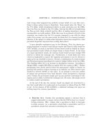
Figure 5.3 illustrates once again the production surface for Equation
(5.4). From our earlier discussion we noted that because of the substi-
tutability of productive inputs, for many productive processes it may be pos-
sible to utilize labor and capital in an infinite number of combinations
(assuming that productive resources are infinitely divisible) to produce, say,
122 units of output. Using the data from Table 5.1, Figure 5.3 illustrates four
such input combinations to produce 122 units of output. It should be noted
once again that efficient production is defined as any input combination on
the production surface. The locus of points II in Figure 5.3 is called an
isoquant.
212 Production

Q
Q
K
L0
3
6
84
122
6
4
I
I
FIGURE 5.3 The production surface
and an isoquant at Q = 122.
Definition:An isoquant defines the combinations of capital and labor (or
any other input combination in n-dimensional space) necessary to produce
a given level of output.
If fractional amounts of labor and capital are assumed, then an infinite
number of such combinations is possible. While Figure 5.3 explicitly shows
only one such isoquant at Q = 122 for Equation (5.4), it is easy to imagine
that as we move along the production surface, an infinite number of such
isoquants are possible corresponding to an infinite number of theoretical
output levels. Projecting downward into capital and labor space, Figure 5.4
illustrates seven such isoquants corresponding to the data presented in
Table 5.1.
Figure 5.4 is referred to as an isoquant map. For any given production
function there are an infinite number of isoquants in an isoquant map. In
general, the function for an isoquant map may be written
(5.16)
where Q

0
denotes a fixed level of output. Solving Equation (5.16) for K
yields
(5.17)
The slope of an isoquant is given by the expression
(5.18)
It measures the rate at which capital and labor can be substituted for
each other to yield a constant rate of output. Equation (5.18) is also referred
dK
dL
g L Q MRTS
KKL
=
()
=<,
0
0
KgLQ=
()
,
0
QfKL
0
=
()
,
Isoquants 213
Labor
0 1 2 3 4 5 6 7 8
0

1
2
3
4
5
6
7
8
Q=50
Q=71
Q=100
Q=122
Q=141
Q=158
Q=187
Capital
FIGURE 5.4 Selected isoquants for the production function Q = 25K
0.5
L
0.5
.
to as the marginal rate of technical substitution of capital for labor
(MRTS
KL
). The marginal rate of technical substitution summarizes the
concept of substitutability discussed earlier. MRTS
KL
says that to maintain
a fixed output level, an increase (decrease) in the use of capital must be
accompanied by a decrease (increase) in the use of labor. It may also be

demonstrated that
(5.19)
Equation (5.19) says that the marginal rate of technical substitution of
capital for labor is the ratio of the marginal product of labor (MP
L
) to the
marginal product of capital (MP
K
).
Definition: If we assume two factors of production, capital and labor, the
marginal rate of technical substitution (MRTS
KL
) is the amount of a factor
of production that must be added (subtracted) to compensate for a reduc-
tion (increase) in the amount of a factor of production to maintain a given
level of output. The marginal rate of technical substitution, which is the
slope of the isoquant, is the ratio of the marginal product of labor to the
marginal product of capital (MP
L
/MP
K
).
To see this, consider Figure 5.5, which illustrates a hypothetical isoquant.
By definition, when we move from point A to point B on the isoquant,
output remains unchanged. We can conceptually break this movement
down into two steps. In going from point A to point C, the reduction in
output is equal to the loss in capital times the contribution of that incre-
mental change in capital to total output (i.e., MP
K
DK < 0). In moving from

point C to point B, the contribution to total output is equal to the incre-
mental increase in labor time marginal product of that incremental increase
MRTS
MP
MP
KL
L
K
=-
214 Production
A
C
I
I
B
L
K
0
M
P
KX
¥ ⌬K
MP
LX
¥ ⌬L
FIGURE 5.5 Slope of an isoquant: marginal rate of technical substitution.
(i.e., MP
L
DL > 0). Since to remain on the isoquant there must be no change
in total output, it must be the case that

(5.20)
Rearranging Equation (5.20) yields
For instantaneous rates of change, Equation (5.20) becomes
(5.21)
Equation (5.21) may also be derived by applying the implicit function
theorem to Equation (5.2).Taking the total derivative of Equation (5.2) and
setting the results equal to zero yields
(5.22)
Equation (5.22) is set equal to zero because output remains unchanged
in moving from point A to point B in Figure 5.5. Rearranging Equation
(5.22) yields
or
Another characteristic of isoquants is that for most production processes
they are convex with respect to the origin. That is, as we move from point
A to point B in Figure 5.5, increasing amounts of labor are required to sub-
stitute for decreased equal increments of capital. Mathematically, convex
isoquants are characterized by the conditions dK/dL < 0 and d
2
K/dL
2
> 0.
That is, as MP
L
declines as more labor is added by the law of diminishing
marginal product, MP
K
increases as less capital is used. This relationship
illustrates that inputs are not perfectly substitutable and that the rate of
substitution declines as one input is substituted for another.Thus, with MP
L

declining and MP
K
increasing, the isoquant becomes convex to the origin.
The degree of convexity of the isoquant depends on the degree of sub-
stitutability of the productive inputs. If capital and labor are perfect sub-
stitutes, for example, then labor and capital may be substituted for each
other at a fixed rate. The result is a linear isoquant, which is illustrated
in Figure 5.6. Mathematically, linear isoquants are characterized by the
dK
dL
MP
MP
L
K
=-
∂∂
∂∂
QL
QK
dK
dL
=
dQ
Q
L
dL
Q
K
dK=
Ê

Ë
ˆ
¯
+
Ê
Ë
ˆ
¯
=
∂
∂
∂
∂
0
dK
dL
MP
MP
MRTS
L
K
KL
=- = <0
D
D
K
L
MP
MP
L

K
=-
-¥=¥MP K MP L
KL
DD
Isoquants 215
conditions dK/dL < 0 and d
2
K/dL
2
= 0. Examples of production processes
in which the factors of production are perfect substitutes might include oil
versus natural gas for some heating furnaces, energy versus time for some
drying processes, and fish meal versus soybeans for protein in feed mix.
Some production processes, on the other hand, are characterized by fixed
input combinations, that is, MRTS
K/L
= KL. This situation is illustrated in
Figure 5.7. Note that the isoquants in this case are “L shaped.” These iso-
quants are discontinuous functions in which efficient input combinations
take place at the corners, where the smallest quantity of resources is used
to produce a given level of output. Mathematically, discontinuous functions
do not have first and second derivatives. Examples of such fixed-input pro-
duction processes include certain chemical processes that require that basic
elements be used in fixed proportions, engines and body parts for automo-
biles, and two wheels and a frame for a bicycle.
216 Production
K
L
0 Q

0
Q
1
Q
2
FIGURE 5.6 Perfect input substitutability.
K
L
0
Q
0
Q
1
Q
2
FIGURE 5.7 Fixed input combinations.
Problem 5.5. The general form of the Cobb–Douglas production function
may be written as:
where A is a positive constant and 0 <a<1, 0 <b<1.
a. Derive an equation for an isoquant with K in terms of L.
b. Demonstrate that this isoquant is convex (bowed in) with respect to the
origin.
Solution
a. An isoquant shows the various combinations of two inputs (say, labor
and capital) that the firm can use to produce a specific level of output.
Denoting an arbitrarily fixed level of output as Q
0
, the Cobb–Douglas
production function may be written
Solving this equation for K in terms of L yields

b. The necessary and sufficient conditions necessary for the isoquant to be
convex (bowed in) to the origin are
The first condition says that the isoquant is downward sloping. The
second condition guarantees that the isoquant is convex with respect to
the origin. Taking the respective derivatives yields
since (-b/a) < 0 and (Q
0
1/a
A
-1/a
L
-b/a-1
) > 0. Taking the second derivative
of this expression, we obtain
since [-(b/a) - 1](-b/a) > 0 and (Q
0
1/a
A
-1/a
L
-b/a-2
) > 0.
Problem 5.6. The Spacely Company has estimated the following produc-
tion function for sprockets:
∂
∂
b
a
b
a

a
a
ba
2
2
0
1
1
2
10
K
L
QAL=-
Ê
Ë
ˆ
¯
-
È
Î
Í
˘
˚
˙
-
Ê
Ë
ˆ
¯
()

>
-

∂
∂
b
a
a
a
ba
K
L
QAL=-
Ê
Ë
ˆ
¯
<
-

0
1
1
1
0
∂
∂
∂
∂
K

L
K
L
<
>
0
0
2
2
KQAL
K
Q
AL
a
b
a
a
ba
=
=
-
-
-
-
0
1
0
1
1
QAKL

0
=
a
b
QAKL=
a
b
Isoquants 217
a. Suppose that Q = 100. What is the equation of the corresponding
isoquant in terms of L?
b. Demonstrate that this isoquant is convex (bowed in) with respect to the
origin.
Solution
a. The equation for the isoquant with Q = 100 is written as
Solving this equation for K in terms of L yields
b. Taking the first and second derivatives of this expression yields
That the first derivative is negative and the second derivative is positive
are necessary and sufficient conditions for a convex isoquant.
LONG-RUN PRODUCTION FUNCTION
RETURNS TO SCALE
It was noted earlier that the long run in production describes the situa-
tion in which all factors of production are variable. A firm that increases its
employment of all factors of production may be said to have increased its
scale of operations. Returns to scale refer to the proportional increase in
output given some equal proportional increase in all productive inputs. As
discussed earlier, constant returns to scale (CRTS) refers to the condition
where output increases in the same proportion as the equal proportional
increase in all inputs. Increasing returns to scale (IRTS) occur when the
increase in output is more than proportional to the equal proportional
increase in all inputs. Decreasing returns to scale (DRTS) occur when the

proportional increase in output is less than proportional increase in all
inputs. To illustrate these relationships mathematically, consider the pro-
duction function
dK
dL
L
dK
dL
L
LL
=<
=- -
()
=
()
=>
-
-
16 0
216
216 32
0
2
2
2
3
33
KL LL
KL
L

05 05
1
105 05
05
2
100 25 100 25 4
4
16

.
=
()
=
()
=
=
()
=
-
-
-
100 25
05 05
= KL

QKL= 25
05 05
218 Production
(5.23)
where output is assumed to be a function of n productive inputs. A func-

tion is said to be homogeneous of degree r if, and only if,
or
(5.24)
where t > 0 is some factor of proportionality. Note the identity sign in
expression (5.24). This is not an equation that holds for only a few points
but for all t, x
1
, x
2
, ,x
n
. This relationship expresses the notion that if all
productive inputs are increased by some factor t, then output will increase
by some factor t
r
, where r > 0. Expression (5.24) is said to be a function that
is homogeneous of degree r.
Returns to scale are described as constant, increasing, or decreasing
depending on whether the value of r is greater than, less than, or equal to
unity. Table 5.2 summarizes these relationships. Constant returns to scale is
the special case of a production function that is homogeneous of degree
one, which is often referred to as linear homogeneity.
Problem 5.7. Consider again the general form of the Cobb–Douglas
production function
where A is a positive constant and 0 <a<1, 0 <b<1. Specify the condi-
tions under which this production function exhibits constant, increasing, and
decreasing returns to scale.
Solution. Suppose that capital and labor are increased by a factor of t.
Then,
The production function exhibits constant, increasing, and decreasing

returns to scale as a+bis equal to, greater than, and less than unity, respec-
f tK tL A tK tL At K t L t AK L t Q,
()
∫
()()
∫∫∫
++
ab
aa
bb ab
a
bab
QAKL
0
=
a
b
tQ ftx tx tx
r
n
∫
()
12
, , ,
ftx tx tx tfx x x
n
r
n12 12
, , , , , ,
()

∫
()
Qfxx x
n
=
()
12
, , ,
Long-Run Production Function 219
TABLE 5.2 Production functions
homogenous of degree r.
r Returns to scale
=1 Constant
>1 Increasing
<1 Decreasing
tively. For example, suppose that a=0.3 and b=0.7 and that capital and
labor are doubled (t = 2). The production function becomes
Since doubling all inputs results in a doubling of output, the production
function exhibits constant returns to scale. This is easily seen by the fact
that a+b=1.
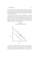
Consider again Equation (5.4).
(5.4)
This Cobb–Douglas production function clearly exhibits constant returns
to scale, since a+b=1. When K = L = 1, then Q = 25. When inputs are
doubled to K = L = 2, then output doubles to Q = 50. This result is illus-
trated in Figure 5.8.
It should be noted that adding exponents to determine whether a
production function exhibits constant, increasing, or decreasing returns to
scale is applicable only to production functions that are in multiplicative
(Cobb–Douglas) form. For all other functional forms, a different approach

is required, as is highlighted in Problem 5.8.
Problem 5.8. For each of the following production functions, determine
whether returns to scale are decreasing, constant, or increasing when capital
and labor inputs are increased from K = L = 1 to K = L = 2.
a. Q = 25K
0.5
L
0.5
b. Q = 2K + 3L + 4KL
c. Q = 100 + 3K + 2L
d. Q = 5K
a
L
b
, where a+b=1
QKL= 25
05 05
AK L A K L AKL Q22 2 2 2 2
03 07
03 03 07 07 03 07 03 07
()()
∫∫∫
+


220 Production
K
L0
Q=25
Q=50

1
1
2
2
FIGURE 5.8 Constant returns to scale.
e. Q = 20K
0.6
L
0.5
f. Q = K/L
g. Q = 200 + K + 2L + 5KL
Solution
a. For K = L = 1,
For K = L = 2 (i.e., inputs are doubled),
Since output doubles as inputs are doubled, this production function
exhibits constant returns to scale. It should also be noted that for
Cobb–Douglas production functions, of which this is one, returns to scale
may be determined by adding the values of the exponents. In this case,
0.5 + 0.5 = 1 indicates that this production function exhibits constant
returns to scale.
b. For K = L = 1,
For K = L = 2,
Since output more than doubles as inputs are doubled, this production
function exhibits increasing returns to scale for the input levels indicated.
c. For K = L = 1,
For K = L = 2,
Since output less than doubles as inputs are doubled, this production
function exhibits decreasing returns to scale for the input levels
indicated.
d. As noted earlier, returns to scale for Cobb–Douglas production

functions may be determined by adding the values of the exponents.This
production function clearly exhibits constant returns to scale.
e. For K = L = 1,
For K = L = 2,
Q =
() ()
=
()()
=20 2 2 20 1 516 1 414 42 872
06 05
.
Q =
() ()
=
()()
=20 1 1 20 1 1 20
06 05
Q =+
()
+
()
=++=100 3 2 2 2 100 6 4 110
Q =+
()
+
()
=++=100 3 1 2 1 100 3 2 105
Q =
()
+

()
+
()()
=++ =22 32 42 2 4 6 16 26
Q =
()
+
()
+
()()
=++=21 31 41 1 2 3 4 9
Q =
() ()
=
()
=25 2 2 25 2 50
05 05 1
Q =
() ()
=25 1 1 25
05 05
Long-Run Production Function 221
Since output more than doubles as inputs are doubled, this produc-
tion function exhibits increasing returns to scale. Since this is a
Cobb–Douglas production function, this result is verified by adding the
values of the exponents (i.e., 0.6 + 0.5 = 1.1). Since this result is greater
than unity, we may conclude that this production function exhibits
increasing returns to scale.
f. For K = L = 1,
For K = L = 2,

Since output does not double (it remains unchanged) as inputs are
doubled, this production function exhibits decreasing returns to scale.
g. For K = L = 1,
For K = L = 2
Since output does not double as inputs are doubled, this production func-
tion exhibits decreasing returns to scale for the input levels indicated.
The reader should verify that when K = L = 100, then Q = 50,500. When
input levels are doubled to K = L = 200, then Q = 200,800. In this case,
a doubling of input usage resulted in an almost fourfold increase in
output (i.e., increasing returns to scale). The important thing to note is
that some production functions may exhibit different returns to scale
depending on the level of input usage. Fortunately, Cobb–Douglas
production functions exhibit the same returns-to-scale characteristics
regardless of the level of input usage.
ESTIMATING PRODUCTION FUNCTIONS
The Cobb–Douglas production function is also the most commonly used
production function in empirical estimation. Consider again Equation (5.3).
(5.3)
Cobb–Douglas production functions may be estimated using ordinary-
least-squares regression methodology.
2
Ordinary least squares regression
QAKL=
a
b
Q =++
()
+
()()
=200 2 2 2 5 2 2 226

Q =++
()
+
()()
=200 1 2 1 5 1 1 208
Q ==
2
2
1
Q ==
1
1
1
222 Production
2
See, for example, W. H. Green, Econometric Analysis,3
rd
ed. (Upper Saddle River: Pren-
tice-Hall, 1997), D. Gujarati, Basic Econometrics,3
rd
ed. (New York: McGraw-Hill, 1995), and
R.Ramanathan,Introductory Econometrics with Applications,4
th
ed. (New York: Dryden, 1998).
analysis is the most frequently used statistical technique for estimating
business and economic relationships. In the case of Equation (5.3), ordinary
least squares may be used to derive estimates of the parameters A, a and
b on the basis observed values of the dependent variable Q and the inde-
pendent variables K and L. To apply the ordinary-least-squares methodol-
ogy, however, the equation to be estimated must be linear in parameters,

which Equation (5.3) clearly is not. This minor obstacle is easily overcome.
Taking logarithms of Equation (5.3) we obtain
(5.25)
The estimated parameter values a and b are no longer slope coefficients
but elasticity values. To begin, recall that y = log x, then
or
Now, taking the first partial derivatives of Equation (5.25) with respect to
K and L, we obtain
and
But ∂log Q =∂Q/Q, ∂ log K =∂K/K, and ∂log L =∂L/L. Therefore
(5.26)
Similarly,
(5.27)
These parameter values represent output elasticities of capital and labor,
while the sum of these parameters is the coefficient of output elasticity
(returns to scale), that is,
(5.28)
Problem 5.9. Consider the following Cobb–Douglas production function
QKL= 56
038 072
eee
Q
KL
=+
∂
∂
∂
∂
∂
∂

be
log
lo
g
Q
L
QQ
LL
Q
L
L
Q
L
==
Ê
Ë
ˆ
¯
Ê
Ë
ˆ
¯
==
∂
∂
∂
∂
∂
∂
ae

log
lo
g
Q
K
QQ
KK
Q
K
K
Q
K
==
Ê
Ë
ˆ
¯
Ê
Ë
ˆ
¯
==
∂
∂
b
log
log
Q
L
=

∂
∂
a
log
log
Q
K
=
dy
dx
x
=
dy
dx x
=
1
log log log logQA K L=+ +ab
Estimating Production Functions 223
a. Demonstrate that the elasticity of production with respect to labor is
0.72.
b. Demonstrate that the elasticity of production with respect to capital is
0.38.
c. Demonstrate that this production function exhibits increasing returns to
scale.
Solution
a. The elasticity of production with respect to labor is
b. The elasticity of production with respect to capital is
c. The Cobb–Douglas production function is
Returns to scale refer to the additional output resulting from an equal
proportional increase in all inputs. If output increases in the same pro-

portion as the increase in all inputs, then the production function exhibits
constant returns to scale. If output increases by a greater proportion than
the equal proportional increase in all inputs, then the production func-
tion exhibits increasing returns to scale. Finally, if output increases by a
lesser proportion than the equal proportional increase in all inputs, the
production function exhibits decreasing returns to scale. To determine
the returns to scale of the foregoing production function, multiply all
factors by some scalar (t > 1), that is,
From this result, it is clear that if inputs are, say, doubled (t = 2), then
output will increase by 2.14 times. From this we conclude that the
production function exhibits increasing returns to scale. In fact, for
Cobb–Douglas production functions, returns to scale are determined by
the sum of the exponents. From the general form of the Cobb–Douglas
production function
56 56 56
56
038 072
038 038 072 072 038 072 038 072
11 038 072 11
tK tL t K t L t K L
tKLtQ
()()
==
==
+
()

.

QKL= 56

038 072
e
∂
∂
K
Q
K
K
Q
KL
K
KL
LK
KL
Q
Q
=
Ê
Ë
ˆ
¯
Ê
Ë
ˆ
¯
=
()
[]
Ê
Ë

ˆ
¯
=
()
==
-
-
03856
56
03856
56
038
038
038 1 072
038 072
062 072
038 072
.

.




e
∂
∂
L
Q
L

L
Q
KL
L
KL
LL
KL
Q
Q
=
Ê
Ë
ˆ
¯
Ê
Ë
ˆ
¯
=
()
[]
Ê
Ë
ˆ
¯
=
()
==
-
-

07256
56
07256
56
072
072
0 38 0 72 1
038 072
038 028
038 072
.

.




224 Production
we can derive Table 5.3
CHAPTER REVIEW
A production function is the technological relationship between the
maximum amount of output a firm can produce with a given combination
of inputs (factors of production). The short run in production is defined as
that period of time during which at least one factor of production is held
fixed. The long run in production is defined as that period of time during
which all factors of production are variable. In the short run, the firm is
subject to the law of diminishing returns (sometimes referred to as the law
of diminishing marginal product), which states that as additional units of a
variable input are combined with one or more fixed inputs, at some point
the additional output (marginal product) will start to diminish.

The short-run production function is characterized by three stages of
production. Assuming that output is a function of labor and a fixed amount
of capital, stage I of production is the range of labor usage in which the
average product of labor (AP
L
) is increasing. Over this range of output, the
marginal product of labor (MP
L
) is greater than the average product of
labor. Stage I ends and stage II begins where the average product of labor
is maximized (i.e., AP
L
= MP
L
).
Stage II of production is the range of output in which the average product
of labor is declining and the marginal product of labor is positive. In other
words, stage II of production begins where AP
L
is maximized and ends with
MP
L
= 0.
Stage III of production is the range of product in which the marginal
product of labor is negative. In stage II and stage III of production, AP
L
>
MP
L
. According to economic theory, production in the short run for a

“rational” firm takes place in stage II.
If we assume two factors of production, the marginal rate of technical
substitution (MRTS
KL
) is the amount of a factor of production that must
be added (subtracted) to compensate for a reduction (increase) in the
QAKL=
a
b
Chapter Review 225
TABLE 5.3 Cobb-Douglas production function and
returns to scale.
a+b Returns to scale
<1 Decreasing
=1 Constant
>1 Increasing
amount of another input to maintain a given level of output. If capital and
labor are substitutable, the marginal rate of technical substitution is defined
as the ratio of the marginal product of labor to the marginal product of
capital, that is, MP
L
/MP
K
.
Returns to scale refers to the proportional increase in output given an
equal proportional increase in all inputs. Since all inputs are variable,
“returns to scale” is a long-run production phenomenon. Increasing returns
to scale (IRTS) occur when a proportional increase in all inputs results in
a more than proportional increase in output. Constant returns to scale
(CRTS) occur when a proportional increase in all inputs results in the same

proportional increase in output. Decreasing returns to scale (DRTS) occur
when a proportional increase in all inputs results in a less than proportional
increase in output.
Another way to measure returns to scale is the coefficient of output elas-
ticity (e
Q
), which is defined as the percentage increase (decrease) in output
with respect to a percentage increase (decrease) in all inputs. The coeffi-
cient of output elasticity is equal to the sum of the output elasticity of labor
(e
L
) and the output elasticity of capital (e
K
), that is, e
Q
=e
L
+e
K
. IRTS occurs
when e
Q
> 1. CRTS occurs when e
Q
= 1. DRTS occurs when e
Q
< 1.
The Cobb–Douglas production function is the most popular specification
in empirical research. Its appeal is largely the desirable mathematical
properties it exhibits, including substitutability between and among inputs,

conformity to the law of diminishing returns to a variable input, and returns
to scale. The Cobb–Douglas production function has several shortcomings,
however, including an inability to show marginal product in stages I and
III.
Most empirical studies of cost functions use time series accounting data,
which present a number of problems. Accounting data, for example, tend
to ignore opportunity costs, the effects of changes in inflation, tax rates,
social security contributions, labor insurance costs, accounting practices, and
so on. There are also other problems associated with the use of accounting
data including output heterogeneity and asynchronous timing of costs.
Economic theory suggests that short-run total cost as a function of
output first increases at an increasing rate, then increases at a decreasing
rate. Cubic cost functions exhibit this theoretical relationship, as well as the
expected “U-shaped” average total, average variable, and marginal cost
curves.
KEY TERMS AND CONCEPTS
Average product of capital (AP
K
) The total product per unit of capital
usage. It is the total product of capital divided by the total amount of
capital employed by the firm.
226 Production
Average product of labor (AP
L
) The total product per unit of labor usage.
It is the total product of labor divided by the total amount of labor
employed by the firm.
Cobb–Douglas production function It may not in practice be possible
precisely to define the mathematical relationship between the output of
a good or service and a set of productive inputs employed by the firm to

produce that good or service. In spite of this, because of certain desir-
able mathematical properties, perhaps the most widely used functional
form to approximate the relationship between the production of a
good or service and a set of productive inputs is the Cobb–Douglas
production function. For the two-input case (capital and labor), the
Cobb–Douglas production function is given by the expression Q =
AK
a
L
b
.
Coefficient of output elasticity The percentage change in the output of a
good or service given a percentage change in all productive inputs. Since
all inputs are variable, the coefficient of output elasticity is a long-run
production concept.
Constant returns to scale (CRTS) The case in which the output of a good
or a service increases in the same proportion as the proportional increase
in all factors of production. Since all inputs are variable, CRTS is a long-
run production concept. In the case of CRTS the coefficient of output
elasticity is equal to unity.
Decreasing returns to scale (DRTS) The case in which the output of a
good or a service increases less than proportionally to a proportional
increase in all factors of production used to produce that good or
service. Since all inputs are variable, DRTS is a long-run production
concept. In the case of DRTS the coefficient of output elasticity is less
than unity.
Factor of production Inputs used in the production of a good or service.
Factors of production are typically classified as land, labor, capital, and
entrepreneurial ability.
Increasing returns to scale (IRTS) The case in which the output of a good

or a service increases more than proportionally to a proportional
increase in all factors of production used to produce that good or service.
Since all inputs are variable, IRTS is a long-run production concept. In
the case of IRTS the coefficient of output elasticity is greater than unity.
Isoquant A curve that defines the different combinations of capital and
labor (or any other input combination in n-dimensional space) necessary
to produce a given level of output.
Law of diminishing marginal product As increasing amounts of a variable
input are combined with one or more fixed inputs, at some point the mar-
ginal product of the variable input will begin to decline. Because at least
one factor of production is held fixed, the law of diminishing returns is
a short-run concept.
Key Terms and Concepts 227
Long run in production In the long run, all factors of production are
variable.
Marginal product of capital (MP
k
) The incremental change in output
associated with an incremental change in the amount of capital usage.
If the production function is given as Q = f(K, L), then the marginal
product of capital is the first partial derivative of the production
function with respect to capital (∂Q/∂K), which is assumed to be
positive.
Marginal product of labor (MP
L
) The incremental change in output asso-
ciated with an incremental change in the amount of labor usage. If the
production function is given as Q = f(K, L), then the marginal product
of labor is the first partial derivative of the production function with
respect to labor (∂Q/∂L), which is assumed to be positive.

Marginal rate of technical substitution (MRTS
KL
) Suppose that output is
a function of variable labor and capital input, Q = f(K, L). The marginal
rate of technical substitution is the rate at which capital (labor) must be
substituted for labor (capital) to maintain a given level of output. The
marginal rate of technical substitution, which is the slope of the isoquant,
is the ratio of the marginal product of labor to the marginal product of
capital (MP
L
/MP
K
).
Production function A mathematical expression that relates the
maximum amount of a good or service that can be produced with a set
of factors of production.
Q = AK
a
L
b
The Cobb–Douglas production function, which asserts that
the output of a good or a service as a multiplicative function of capital
(K) and labor (L).
Short run in production That period of time during which at least one
factor of production is constant.
Stage I of production Assuming that output is a function of variable
labor and fixed capital, this is the range of labor usage in which the
average product of labor is increasing. Over this range of output, the
marginal product of labor is greater than the average product of labor.
Stage I ends, and stage II begins, where the average product of labor

is maximized (i.e., AP
L
= MP
L
). According to economic theory, produc-
tion in the short run for a “rational” firm takes place in stage II of
production.
Stage II of production Assuming that output is a function of variable
labor and fixed capital, this is the range of output in which the average
product of labor is declining and the marginal product of labor is posi-
tive. Stage II of production begins where AP
L
is maximized, and ends
with MP
L
= 0.
Stage III of production Assuming that output is a function of variable
labor and fixed capital, this is the range of production in which the mar-
ginal product of labor is negative.
228 Production
Total product of capital Assuming that output is a function of variable
capital and fixed labor, this is the total output of a firm for a given level
of labor input.
Total product of labor Assuming that output is a function of variable
labor and fixed capital, this is the total output of a firm for a given level
of labor input.
CHAPTER QUESTIONS
5.1 What is the difference between a production function and a total
product function?
5.2 What is meant by the short run in production?

5.3 What is meant by the long run in production?
5.4 What is the total product of labor? What is the total product of
capital? Are these short-run or long-run concepts?
5.5 Suppose that output is a function of labor and capital. Assume that
labor is the variable input and capital is the fixed input. Explain the law of
diminishing marginal product. How is the law of diminishing marginal
product reflected in the total product of labor curve?
5.6 Assume that a production function exhibits the law of diminishing
marginal product. What are the signs of the first and second partial deriv-
atives of output with respect to variable labor input?
5.7 Suppose that the total product of labor curve exhibits increasing,
diminishing and negative marginal product. Describe in detail the shapes
of the marginal product and average product curves.
5.8 Suppose that the total product of labor curve exhibits only dimin-
ishing marginal product. Describe in detail the shapes of the marginal
product and average product curves.
5.9 Explain the difference between the law of diminishing marginal
product and decreasing returns to scale.
5.10 Suppose that output is a function of labor and capital. Define the
output elasticity of variable labor input. Define the output elasticity of vari-
able capital input. What is the sum of the output elasticity of variable labor
and variable capital input?
5.11 Suppose that a firm’s production function is Q = 75K
0.4
L
0.7
. What is
the value of the output elasticity of labor? What is the value of the output
elasticity of capital? Does this firm’s production function exhibit constant,
increasing, or decreasing returns to scale?

5.12 Define “marginal rate of technical substitution.”
5.13 Suppose that output is a function of labor and capital. Diagram-
matically, what is the marginal rate of technical substitution?
5.14 Explain the difference between perfect and imperfect substi-
tutability of factors of production.
Chapter Questions 229
5.15 What does an “L-shaped” isoquant illustrate? Can you give an
example of a production process that would exhibit an “L-shaped” iso-
quant?
5.16 What does a linear isoquant illustrate?
5.17 Isoquants cannot intersect. Do you agree? Explain.
5.18 The degree of convexity of an isoquant determines the degree of
substitutability of factors of production. Do you agree? Explain.
5.19 Suppose that output is a function of capital and labor input.Assume
that the production function exhibits imperfect substitutability between the
factors of production. What, if anything, can you say about the values of the
first and second derivatives of the isoquant?
5.20 Suppose that a firm’s production function is Q = KL
-1
. Does this
production function exhibit increasing, decreasing, or constant returns to
scale? Explain.
5.21 Define each of the following:
a. Stage I of production
b. Stage II of production
c. Stage III of production
5.22 When the average product of labor is equal to the marginal product
of labor, the marginal product of labor is maximized. Do you agree?
Explain.
5.23 Suppose that output is a function of labor and capital input. The

slope of an isoquant is equal to the ratio of the marginal products of capital
and labor. Do you agree? Explain.
5.24 Suppose that output is a function of labor and capital input. If a
firm decides to reduce the amount of capital employed, how much labor
should be hired to maintain a given level of output?
5.25 What is the ratio of the marginal product of labor to the average
product of labor?
5.26 Isoquants may be concave with respect to the origin. Do you agree?
Explain.
5.27 Firms operate in the short run and plan in the long run. Do you
agree? Explain.
5.28 Describe at least three desirable properties of Cobb–Douglas pro-
duction functions.
5.29 What is the relationship between the average product of labor and
the marginal product of labor?
5.30 What is the coefficient of output elasticity?
5.31 Suppose that output is a function of labor and capital input.
Suppose further that the corresponding isoquant is linear.These conditions
indicate that labor and capital are not substitutable for each other. Do you
agree? Explain.
5.32 Suppose that output is a function of labor and capital input.
Suppose further that capital and labor must be combined in fixed propor-
230 Production
tions. These conditions indicate that returns to scale are constant. Do you
agree? Explain.
5.33 An increase in the size of a company’s labor force resulted in
an increase in the average product of labor. For this to happen, the firm’s
total output must have increased. Do you agree? Explain.
5.34 An increase in the size of a company’s labor force will result in a
shift of the average product of labor curve up and to the right. This indi-

cates that the company is experiencing increasing returns to scale. Do you
agree? Explain.
5.35 Suppose that output is a function of labor and capital input and
exhibits constant returns to scale. If a firm doubles its use of both labor and
capital, the total product of labor curve will become steeper. Do you agree?
Explain.
CHAPTER EXERCISES
5.1 Suppose that the production function of a firm is given by the
equation
where Q represents units of output, K units of capital, and L units of labor.
What is the marginal product of labor and the marginal product of capital
at K = 40 and L = 10?
5.2 A firm’s production function is given by the equation
where Q represents units of output, K units of capital, and L units of
labor.
a. Does this production function exhibit increasing, decreasing, or con-
stant returns to scale?
b. Suppose that Q = 1,000. What is the equation of the corresponding
isoquant in terms of labor?
c. Demonstrate that this isoquant is convex with respect to the origin.
5.3 Determine whether each of the following production functions
exhibits increasing, decreasing, or constant returns to scale for K = L = 1
and K = L = 2.
a. Q = 10 + 2L
2
+ K
3
b. Q = 5 + 10K + 20L + KL
c. Q = 500K
0.7

L
0.1
d. Q = K + L + 5LK
5.4 Suppose that a firm’s production function has been estimated as
QKL= 5
05 05
QKL= 100
03 08
QKL= 2
55
Chapter Exercises 231
where Q is units of output, K is machine hours, and L is labor hours.
Suppose that the amount of K available to the firm is fixed at 100 machine
hours.
a. What is the firm’s total product of labor equation? Graph the total
product of labor equation for values L = 0 to L = 200.
b. What is the firm’s marginal product of labor equation? Graph the
marginal product of labor equation for values L = 0 to L = 200.
c. What is the firm’s average product of labor equation? Graph
the average product of labor equation for values L = 0 to
L = 200.
5.5 Suppose that a firm’s short-run production function has been
estimated as
where Q is units of output and L is labor hours.
a. Graph the production function for values L = 0 to L = 200.
b. What is the firm’s marginal product of labor equation? Graph the
marginal product of labor equation for values L = 0 to L = 200.
c. What is the firm’s average product of labor equation? Graph the
average product of labor equation for values L = 0 to L = 200.
5.6 Lothian Company has estimated the following production function

for its product lembas
where Q represents units of output, K units of capital, and L units of
labor. What is the coefficient of output elasticity? What are the returns to
scale?
5.7 The average product of labor is given by the equation
a. What is the equation for the total product of labor (TP
L
)?
b. What is the equation for the marginal product of labor (MP
L
)?
c. At what level of labor usage is AP
L
= MP
L
?
SELECTED READINGS
Brennan, M. J., and T. M. Carrol. Preface to Quantitative Economics & Econometrics, 4th ed.
Cincinnati, OH: South-Western Publishing, 1987.
Cobb, C.W., and P. H. Douglas.“A Theory of Production.” American Economic Review March
(1928), pp. 139–165.
Douglas, P. H. “Are There Laws of Production?” American Economic Review, March (1948),
pp. 1–41.
———. “The Cobb–Douglas Production Function Once Again: Its History, Its Testing, and
Some New Empirical Values.” Journal of Political Economy, October (1984), pp. 903–915.
AP L L
L
=+ -600 200
2
QKL= 10

03 07
QL L L=+ -2 0 4 0 002
23

232 Production
Glass, J. C. An Introduction to Mathematical Methods in Economics. New York: McGraw-Hill,
1980.
Henderson, J. M., and R. E. Quandt. Microeconomic Theory: A Mathematical Approach, 3rd
ed. New York: McGraw-Hill, 1980.
Maxwell, W. D. Production Theory and Cost Curves. Applied Economics, 1, August (1969), pp.
211–224.
Silberberg, E. The Structure of Economics: A Mathematical Approach, 2nd ed. New York:
McGraw-Hill, 1990.
Walters,A. A. Production and Cost Functions: An Econometric Survey. Econometrica, January
(1963), pp. 1–66.
Selected Readings 233
This Page Intentionally Left Blank
6
Cost
235
In Chapter 5 we reviewed the theoretical implications of the technolog-
ical process whereby factors of production are efficiently transformed into
goods and services for sale in the market. The production function defines
the maximum rate of output per unit of time obtainable from a given set
of productive inputs. The production function, however, was presented as a
purely technological relationship devoid of any behavioral assertions
underlying motives of management. The optimal combination of inputs
used in the production process will differ depending on the firm’s organi-
zational objectives. The objective of profit maximization, for example, may
require that the firm use one set of productive resources, while maximiza-

tion of revenue or market share may require a completely different set.
The substitutability of inputs in the production process indicates that any
given level of output may be produced with multiple factor combinations.
Deciding which of these combinations is optimal not only depends on a
well-defined organizational objective but also requires that management
attempt to achieve this objective while constrained by a limited operating
budget and constellation of factor prices. Changes in the budget constraints
or factor prices will alter the optimal combination of inputs. The purpose
of this chapter is to bridge the gap between production as a purely tech-
nological relationship and the cost of producing a level of output to achieve
a well-defined organizational objective.
THE RELATIONSHIP BETWEEN PRODUCTION
AND COST
The cost function of a profit-maximizing firm shows the minimum cost
of producing various output levels given market-determined factor prices
and the firm’s budget constraint. Although largely the domain of accoun-
tants, the concept of cost to an economist carries a somewhat different con-
notation. As already discussed in Chapter 1, economists generally are
concerned with any and all costs that are relevant to the production process.
These costs are referred to as total economic costs. Relevant costs are all
costs that pertain to the decision by management to produce a particular
good or service.
Total economic costs include the explicit costs associated with the day-
to-day operations of a firm, but also implicit (indirect) costs. All costs, both
explicit and implicit, are opportunity costs. They are the value of the next
best alternative use of a resource. What distinguishes explicit costs from
implicit costs is their “visibility” to the manager. Explicit costs are some-
times referred to as “out-of-pocket” costs. Explicit costs are visible expen-
ditures associated with the procurement of the services of a factor of
production. Wages paid to workers are an example of an explicit cost.

By contrast, implicit costs are, in a sense, invisible: the manager will not
receive an invoice for resources supplied or for services rendered.To under-
stand the distinction, consider the situation of a programmer who is weigh-
ing the potential monetary gains from leaving a job at a computer software
company to start a consulting business. The programmer must consider not
only the potential revenues and out-of-pocket expenses (explicit costs) but
also the salary forgone by leaving the computer company. The programmer
will receive no bill for the services he or she brings to the consulting
company, but the forgone salary is just as real a cost of running a consult-
ing business as the rent paid for office space. As with any opportunity cost,
implicit costs represent the value of the factor’s next best alternative use
and must therefore be taken into account. As a practical matter, implicit
costs are easily made explicit. In the scenario just outlines, the programmer
can make the forgone salary explicit by putting himself or herself “on the
books” as a salaried employee of the consulting firm.
SHORT-RUN COST
The theory of cost is closely related to the underlying production tech-
nology. We will begin by assuming that the firm’s short-run total cost (TC)
of production is given by the expression
(6.1)
As we discussed in Chapter 5, the short run in production is defined as that
period of time during which at least one factor of production is held at some
fixed level. Assuming only two factors of production, capital (K) and labor
(L), and assuming that capital is the fixed factor (K
0
), then Equation (6.1)
may be written
TC f Q=
()
236 Cost