Learning in Partially Observable Markov Decision Processes
Bạn đang xem bản rút gọn của tài liệu. Xem và tải ngay bản đầy đủ của tài liệu tại đây (816.47 KB, 56 trang )
Graduate School ETD Form 9
(Revised 12/07)
PURDUE UNIVERSITY
GRADUATE SCHOOL
Thesis/Dissertation Acceptance
This is to certify that the thesis/dissertation prepared
By
Entitled
For the degree of
Is approved by the final examining committee:
Chair
To the best of my knowledge and as understood by the student in the Research Integrity and
Copyright Disclaimer (Graduate School Form 20), this thesis/dissertation adheres to the provisions of
Purdue University’s “Policy on Integrity in Research” and the use of copyrighted material.
Approved by Major Professor(s): ____________________________________
____________________________________
Approved by:
Head of the Graduate Program Date
Mohit Sachan
Learning in Partially Observable Markov Decision Processes
Master of Science
Snehasis Mukhopadhyay
Rajeev Raje
Mohammad Al Hasan
Snehasis Mukhopadhyay
Shiaofen Fang
07/02/2012
Graduate School Form 20
(Revised 9/10)
PURDUE UNIVERSITY
GRADUATE SCHOOL
Research Integrity and Copyright Disclaimer
Title of Thesis/Dissertation:
For the degree of
Choose your degree
I certify that in the preparation of this thesis, I have observed the provisions of Purdue University
Executive Memorandum No. C-22, September 6, 1991, Policy on Integrity in Research.*
Further, I certify that this work is free of plagiarism and all materials appearing in this
thesis/dissertation have been properly quoted and attributed.
I certify that all copyrighted material incorporated into this thesis/dissertation is in compliance with the
United States’ copyright law and that I have received written permission from the copyright owners for
my use of their work, which is beyond the scope of the law. I agree to indemnify and save harmless
Purdue University from any and all claims that may be asserted or that may arise from any copyright
violation.
______________________________________
Printed Name and Signature of Candidate
______________________________________
Date (month/day/year)
*Located at />Learning in Partially Observable Markov Decision Processes
Master of Science
Mohit Sachan
07/02/2012
LEARNING IN
PARTIALLY OBSERVABLE MARKOV DECISION PROCESSES
A Thesis
Submitted to the Faculty
of
Purdue University
by
Mohit Sachan
In Partial Fulfillment of the
Requirements for the Degree
of
Master of Science
August 2012
Purdue University
Indianapolis, Indiana
ii
This work is dedicated to my family and friends.
iii
ACKNOWLEDGMENTS
I am heartily thankful to my supervisor, Dr. Snehasis Mukhopadhyay, whose en-
couragement, guidance and support from the initial to the final level enabled me to
develop an understanding of the subject. He patiently provided the vision, encour-
agement and advise necessary for me to proceed through the masters program and
complete my thesis.
Special thanks to my committee, Dr. Rajeev Raje and Dr. Mohammad Al Hasan for
their support, guidance and helpful suggestions. Their guidance has served me well
and I owe them my heartfelt appreciation.
Thank you to all my friends and well-wishers for their good wishes and support. And
most importantly, I would like to thank my family for their unconditional love and
support.
iv
TABLE OF CONTENTS
Page
LIST OF FIGURES . . . . . . . . . . . . . . . . . . . . . . . . . . . . . . . v
ABSTRACT . . . . . . . . . . . . . . . . . . . . . . . . . . . . . . . . . . . vi
1 INTRODUCTION . . . . . . . . . . . . . . . . . . . . . . . . . . . . . . 1
1.1 Organization of thesis . . . . . . . . . . . . . . . . . . . . . . . . . . 10
2 BACKGROUND LITERATURE . . . . . . . . . . . . . . . . . . . . . . 11
2.1 POMDP value iteration . . . . . . . . . . . . . . . . . . . . . . . . 12
2.2 POMDP policy iteration . . . . . . . . . . . . . . . . . . . . . . . . 14
2.3 The Q
MDP
Value Method . . . . . . . . . . . . . . . . . . . . . . . 14
2.4 Replicated Q-Learning . . . . . . . . . . . . . . . . . . . . . . . . . 15
2.5 Linear Q-Learning . . . . . . . . . . . . . . . . . . . . . . . . . . . 16
3 STATE ESTIMATION . . . . . . . . . . . . . . . . . . . . . . . . . . . . 18
4 LEARNING IN POMDP USING TREE . . . . . . . . . . . . . . . . . . 30
4.1 Automata Games and Decision Making in POMDP . . . . . . . . . 33
4.2 Learning as a Control Strategy for POMDP . . . . . . . . . . . . . 33
4.2.1 The automaton updating procedure . . . . . . . . . . . . . . 34
4.2.2 Ergodic finite Markov chain property . . . . . . . . . . . . . 36
4.2.3 Convergence . . . . . . . . . . . . . . . . . . . . . . . . . . . 38
5 RESULTS . . . . . . . . . . . . . . . . . . . . . . . . . . . . . . . . . . . 40
6 CONCLUSION AND FUTURE WORK . . . . . . . . . . . . . . . . . . 44
LIST OF REFERENCES . . . . . . . . . . . . . . . . . . . . . . . . . . . . 46
v
LIST OF FIGURES
Figure Page
1.1 Markov Process Example . . . . . . . . . . . . . . . . . . . . . . . . . . 1
1.2 Hidden Markov Model Example . . . . . . . . . . . . . . . . . . . . . . 2
1.3 Markov Decision Process Example . . . . . . . . . . . . . . . . . . . . 3
1.4 Partially Observable Markov Decision Process Example . . . . . . . . . 4
1.5 Comparison of different markov models . . . . . . . . . . . . . . . . . . 5
3.1 POMDP Agent decomposition . . . . . . . . . . . . . . . . . . . . . . . 18
3.2 State Estimation . . . . . . . . . . . . . . . . . . . . . . . . . . . . . . 24
3.3 POMDP Example diagram . . . . . . . . . . . . . . . . . . . . . . . . . 26
3.4 State Estimation Example . . . . . . . . . . . . . . . . . . . . . . . . . 27
5.1 Normalized long term reward in a POMDP with 6 states over 200
iterations . . . . . . . . . . . . . . . . . . . . . . . . . . . . . . . . . . 41
5.2 Normalized long term reward in a POMDP with 4 states over 200
iterations . . . . . . . . . . . . . . . . . . . . . . . . . . . . . . . . . . 41
5.3 Normalized long term reward in a POMDP with 4 states over 1000
iterations . . . . . . . . . . . . . . . . . . . . . . . . . . . . . . . . . . 42
5.4 Normalized long term reward in a POMDP with 6 states over 1000
iterations . . . . . . . . . . . . . . . . . . . . . . . . . . . . . . . . . . 42
5.5 Normalized long term reward in a POMDP with 6 states over 1000
iterations . . . . . . . . . . . . . . . . . . . . . . . . . . . . . . . . . . 43
vi
ABSTRACT
Sachan, Mohit. M.S., Purdue University, August 2012. Learning in Partially
Observable Markov Decision Processes. Major Professor: Snehasis Mukhopadhyay.
Learning in Partially Observable Markov Decision process (POMDP) is motivated by
the essential need to address a number of realistic problems. A number of methods
exist for learning in POMDPs, but learning with limited amount of information about
the model of POMDP remains a highly anticipated feature. Learning with minimal
information is desirable in complex systems as methods requiring complete informa-
tion among decision makers are impractical in complex systems due to increase of
problem dimensionality.
In this thesis we address the problem of decentralized control of POMDPs with un-
known transition probabilities and reward. We suggest learning in POMDP using
a tree based approach. States of the POMDP are guessed using this tree. Each
node in the tree has an automaton in it and acts as a decentralized decision maker
for the POMDP. The start state of POMDP is known as the landmark state. Each
automaton in the tree uses a simple learning scheme to update its action choice and
requires minimal information. The principal result derived is that, without proper
knowledge of transition probabilities and rewards, the automata tree of decision mak-
ers will converge to a set of actions that maximizes the long term expected reward
per unit time obtained by the system. The analysis is based on learning in sequential
stochastic games and properties of ergodic Markov chains. Simulation results are
presented to compare the long term rewards of the system under different decision
control algorithms.
1
1 INTRODUCTION
A Markov chain is a mathematical system that undergoes transitions from one state
to another, between a finite or countable number of possible states. It is a random
process characterized as memoryless: the next state depends only on the current state
and not on the sequence of events that preceded it. This specific kind of “memory-
lessness” is called the Markov property [1].
Following is an example of Markov chain.
Figure 1.1. Markov Process Example
In Figure 1.1 there are 2 states S1 and S2 in Markov chain. The agent makes a
transition from S1 to S2 with probability p = 0.9 and remain in the same state S1
with probability p = 0.1. Similarly when in state S2, it makes transition to state
S1 with probability 0.8 and remains in same state S2 with probability p = 0.2. The
transition to the next state depends only on the current state of the agent.
2
If we add uncertainty to a markov chain in the form that we cannot see what state we
are currently in we get a hidden markov model (HMM). In a regular Markov model,
the state is directly visible to the observer, and therefore the state transition probabil-
ities are the only parameters whereas in a HMM, the state is not directly visible, but
output, dependent on the state, is visible. Each state has a probability distribution
over the possible output observations. Therefore the sequence of observations gen-
erated by an HMM gives some information about the sequence of states. HMM are
especially known for their application in pattern recognition such as speech, handwrit-
ing [2], gesture recognition [3], part-of-speech tagging [4], musical score following [5],
partial discharges [6] and bioinformatics.
Figure 1.2. Hidden Markov Model Example
In Figure 1.2 of Hidden Markov Model, we have two states S1 and S2. The agent
makes a transition from S1 to S2 with probability p = 0.9 and remains in the same
state S1 with probability p = 0.1. Similarly from state S2, the agent makes a transi-
tion to state S1 with probability 0.8 and remains in same state S2 with probability
p = 0.2. But the states are not visible to the agent directly, instead it sees an obser-
vation symbol O1 with probability p = 0.75 when it is in state S1 and observation
symbol O2 with probability p = 0.8 when in state S2.
3
Addition of controllable actions in each state in a Markov chain gives us a Markov
Decision Process (MDP). In MDP, the next state is determined by the current state
and an action. The Markov Property holds for MDP also as it is memoryless and
depends only on current state and current action. Markov Decision Processes are
an extension of Markov chains; the difference being the addition of actions in each
state (allowing choices) and the assignment of rewards or penalty for taking an action
(adding motivation) in each state. If there is only one action available for each state
and all rewards are zero, a Markov decision process reduces to a Markov chain.
Following is an example of Markov Decision Process.
Figure 1.3. Markov Decision Process Example
In Figure 1.3 of MDP, we have two states S1 and S2. There are two actions A1 and
A2 available in each of the states. In state S1 if agent takes action A1, it moves
to state S2 with probability p = 0.7 and if it takes action A2 it moves to state S2
with probability p = 0.9. Similarly at state S2 the agent moves to state S1 with
probability p = 0.6 if it takes action A1 and it moves to S1 with probability p = 0.8
if it takes action A2.
4
Further introduction of uncertainty in Markov Decision Processes gives rise to Par-
tially Observable Markov Decision Processes (POMDPs). In POMDP we cannot see
which state we are currently in, however each state emits observation symbols. Thus
the only way to guess the present state is through the emitted observation symbols.
Following is an example of a Partially Observable Markov Decision Process.
Figure 1.4. Partially Observable Markov Decision Process Example
The POMDP in Figure 1.4 contains two states S1 and S2. Each state has choice of
two actions A1 and A2 available. The agent moves from S1 to S2 with probability
p = 0.7, if it chooses action A1 and if it choose A2 at S1 it moves to S2 with
probability p = 0.9. Similarly at state S2 the agent moves to state S1 with probability
p = 0.6, if it takes action A1 and moves to state S1 with probability p = 0.8, if it
takes action A2.
5
The agent does not see which state it is in instead it see the observation symbol emit-
ted by the states. State S1 emits observation symbol O1 with probability p = 0.75
and state S2 emits observation symbol O2 with probability p = 0.8.
The following diagram outlines the difference between different Markov models.
Figure 1.5. Comparison of different Markov models
In real life, decisions that humans and computers make on all levels usually have two
types of impacts:
• They cost or save time, money, or other resources, or they bring revenues,
• They have an impact on the future, by influencing the dynamics.
In many situations, decisions with the largest immediate profit may not be good in
view of future events. MDPs model this paradigm and provide results on the struc-
ture and existence of good policies and on methods for their calculation. MDPs have
attracted the attention of many researchers because they are important both from
the practical and the intellectual point of view. MDPs provide tools for the solution
of important real-life problems [7] and give a mathematical framework for modeling
6
decision-making in situations where outcomes are partly random and partly under the
control of a decision maker. They have proven to be useful particularly in a variety
of sequential planning applications where it is crucial to account for uncertainty in
the process [8].
A Markov decision process (MDP) is defined by the following 4 elements:
• A finite number of states of the environment Φ = {φ
1
, φ
2
, , φ
n
},
• A finite set of actions available α = {α
1
, α
2
, , α
k
}
(Alternatively, α
i
is the finite set of actions available from state φ
i
.),
• A payoff function
R : Φ × Φ × α → {−1, 0, 1}
such that r
i
j
(k) = R(φ
i
, φ
j
, α) is the immediate reward (or expected immedi-
ate reward) received after transition from state φ
i
to state φ
j
using action α.
(Here -1 corresponds to penalty, 0 corresponds to no feedback, 1 corresponds to
reward),
• A state transition probability function
P : Φ × Φ × α → (0, 1)
Where p
i
j
= P (φ
i
, φ
j
, α) determines the probability that action α in state φ
i
at time t will lead to state φ
j
at time t + 1. P
α
(φ
i
, φ
j
) = P r(φ
t+1
= φ
j
|φ
t
=
φ
i
, α
t
= α).
The objective of learning algorithm in the MDP is to determine a policy π : Φ → α
which results in maximum long term reward.
A Partially Observable Markov Decision Process (POMDP) is further generalization
of a Markov Processes. A POMDP is similar to an MDP; we have a set of states, a set
of actions, and transition among states and finally get rewards as effect of transition.
The actions effect on the state in a POMDP is exactly the same as in an MDP. The
7
difference being we can’t observe the current state of the process so in a POMDP we
add a set of observations to the model. Now instead of directly observing the current
state, the state gives us an observation token, which provides a hint about the state
in which the process may reside. These observations are generally probabilistic; so
we need to also specify an observation function. This observation function tells us
the probability of each observation for each state in the model. The observation like-
lihood can also be made to depend on the action if needed.
An Agent in artificial intelligence (AI) is a system that perceives its environment and
takes action that maximizes its chance of success. One of the goals of AI is to design
an agent which can interact with an environment so as to maximize some reward
function.
A POMDP models an agent decision process where system dynamics are determined
by an MDP, but the agent cannot directly observe the underlying state. To know
what state it is in, it maintains a probability distribution over the set of possible
states, based on a set of observations and observation probabilities, and the underly-
ing MDP. The POMDP framework is a general framework and it can model a variety
of real-world sequential decision processes. This model augments a well-researched
framework of Markov decision processes (MDPs) [8], [9] to situations where an agent
cannot reliably identify the underlying environment state. The POMDP formalism
is very general and powerful, extending the application of MDPs to many realistic
problems [10].
A POMDP is defined as a tuple (Φ, α, O, T, Ω, R), where
• S is a set of states Φ = {φ
1
, φ
2
, , φ
n
},
• A is a set of actions α = {α
1
, α
2
, , α
k
},
• O is a set of observations O = {o
1
, o
2
, , o
m
},
8
• T is a set of conditional transition probabilities, P (φ
j
|φ
i
, α),
• Ω is a set of conditional observation probabilities P (O|Φ),
• R : Φ × Φ × α → {−1, 0, 1} is the reward function.
At each time period, the environment is in some state φ
i
∈ Φ. The agent takes an
action α
i
r
i
∈ α, which causes the environment to transition to state φ
j
with probabil-
ity T (φ
j
|φ
i
, α
i
r
i
). Finally, the agent receives a reward with expected value, say r
i
j
(k),
and the process repeats. The difficulty is that the agent does not know the exact
state it is in. Instead, it must maintain a probability distribution, known as the belief
state, over the possible states Φ. An agent needs to update its belief upon taking the
action α and observing O. Since the state is Markovian, maintaining a belief over
the states solely requires knowledge of the previous belief state, the action taken, and
the current observation. The operation is denoted b = τ (b, α
i
, o). Where b is the
present belief state and it depends on previous belief state b, action taken α
i
and the
observation symbol o seen in the transition.
POMDP problems with various performance criteria have been posed and the uses of
dynamic programming methods to determine the optimal policy are well known [9],
[11]. However, several important factors have limited the applicability of this type of
approach. First, the computation becomes burdensome when the number of states
is large. Secondly, There is no way to guess the current state based on observation
symbol with certainty. Third, the information about the model that is required for an
approach such as dynamic programming is not available. Specifically, transition prob-
abilities and corresponding rewards associated with various actions may be unknown
at the time control begun or may change during system operation. This leads to a
new adaptive problem in which, typically, parameters are estimated and, using a sepa-
ration principle, the subsequent estimates are used to update control actions [12], [13].
9
Due to the generality of POMDPs, it entails a high computational cost to solve it.
The problem of finding optimal policies for finite-horizon POMDPs has been proven
to be PSPACE-complete [14]. Because of the intractability of current solution algo-
rithms, especially those that use dynamic programming to construct (approximately)
optimal value functions [15], [16], the application of POMDPs remains limited to very
small problems.
We suggest a method that addresses learning problem is POMDP and avoids a lot of
computational difficulty. The approach is different from many other currently used
approaches as no dependence on an unknown parameter is assumed. We suggest a
learning approach based on a tree, in which each node contains a learning automaton
(LA). The root node of the tree is the only known start state (Landmark state) of
POMDP. Each node in the tree has child nodes corresponding to actions available
and observation symbol emitted by the states. Each node in this LA tree corresponds
to a POMDP state. Each state in POMDP chooses its action through a correspond-
ing LA in the tree independently without the knowledge of outer world. There is no
knowledge that other agents exist or indeed that the world is an N-state POMDP
whose transition probabilities and corresponding rewards depend on actions chosen.
Each LA in the tree tries to improve its own performance by choosing a favorable
action. It chooses an action and waits for a response. No information is passes until
the process returns to the same node again. Once the process returns to the same
node the LA receives the required information and updates its action.
There is no need for explicit synchronization of different LAs in the tree. Action
at each LA node is updated only when the process returns to the same state. The
updating is done via a simple learning scheme. This scheme uses a cumulative reward
obtained from a given action normalized by the total elapsed time under that action
as its environmental response.
10
The result is that individuals operating in nearly total ignorance of their surroundings
can implicitly coordinate themselves to lead to optimal group behavior. This result
is based on a result on learning in N-player identical payoff games [17].
The Landmark based approach is practical and not limiting because in most POMDP
problems we have information available about the starting states and starting state
may have some sensor that will make sure about the state when the process returns to
this state again. The Landmark state relies on the availability of sensor information
to make sure of the state.
1.1 Organization of thesis
The thesis is broadly divided into two parts: state estimation in POMDP using a tree
and then learning in POMDP using that state estimation tree. Chapter 2 will discuss
the background necessary for understanding this thesis and some current solution to
POMDP problems. In chapter 3, state estimation will be discussed in detail. We
will describe how a state in POMDP corresponds to a node in our tree. Chapter 4
will discuss the learning algorithm using learning automata in state estimation tree
in details and how each node in the tree updates its actions. Chapter 5 will show the
results and simulation of the learning algorithm on a simple POMDP problem and
will compare the results with other algorithms. Chapter 6 concludes our work and
suggests future work.
11
2 BACKGROUND LITERATURE
This thesis draws motivation from the work done by Richard M. Wheeler and Kumpati
S. Narendra which describes method for decentralized learning in Markov Decision
Processes [17]. This thesis takes similar approach for learning in POMDP. In [17],
they address adaptive problem in MDP where transition probabilities may change
during the MDP process. [17] suggests model setting of myopic local agents, one lo-
cated at each state of MDP, which is unaware of the surrounding world. There is no
knowledge that other agents exist or indeed that the world is an N- state Markov chain
whose transition probabilities and corresponding rewards depend on actions chosen.
The approach works well for MDPs but cannot be used when there is uncertainty in
states as we dont know what state we are currently in.
A policy is a set of rules that define what action to take in what state in an MDP
or POMDP such that long term rewards are maximized. In order to find a policy or
decision control in POMDP we need some form of memory for our agent to choose
actions correctly [18]. We need to maintain a probability distribution over the states
of underlying environment. This distribution is called belief state and is normally
represented as b(s) to indicate what agent believes about its current state. Using
the POMDP model the belief states are updated based on the agents action and
observations such that the belief states correspond exactly to the state occupation
probabilities. Since the agents belief state is an accurate summary of all relevant past
information it can be used by agent to choose optimal action. Belief states in combi-
nation with the updating rule form a completely observable MDP with a continuous
state space.
12
The agent’s policy π specifies an action α = π(b) for any belief b. The optimal policy
π
∗
yields the highest expected reward value for each belief state and is represented by
optimal value function V
∗
. A powerful result of [15] is that optimal value function for
any POMDP can be approximated arbitrarily well by a piecewise linear and convex
function (PWLC). There exist a class of POMDP that has a value function exactly
as PWLC [15]. These results apply to optimal Q function, where Q function for
action α, Q
α
(b) is the expected reward for a policy. For the Q function Q
α
(b) the
policy takes action α in belief state b and behaves optimally. To behave optimally,
the agent chooses an action α that has the largest Q value for the given belief state.
The representation simplicity of PWLC functions makes them convenient. A PWLC
function Q
α
(b) can be written simply as
Q
α
(b) = max
q∈L
α
q.b (2.1)
where L
α
is a finite set of S dimensional vector. So Q
α
(b) is the maximum of a finite
set of linear functions of b. To solve a POMDP using Q function we can temporar-
ily ignore the observation model and make use of the Q values of the underlying MDP.
Some of the methods used to solve POMDP are discussed in the following sections.
2.1 POMDP value iteration
Value iteration for MDPs is a standard method of maximizing long term reward
and finding the optimal infinite horizon policy π
∗
using a sequence of optimal finite
horizon value functions V
0
∗, V
1
∗, V
2
∗ V
t
∗ [9]. The difference between the optimal
value function and the optimal t-horizon value function goes to zero as t goes to
infinity:
lim
t→∞
max
s∈S
| V
∗
(s) − V
t
∗
(s) | = 0. (2.2)
13
Any POMDP can be reduced to a continuous belief-state MDP. Therefore, value
iteration can also be used to calculate optimal infinite horizon POMDP policies as
following:
• Initialize t = 0 and V
0
(b) = 0 for all b ∈ B
• While max
b∈B
| V
t+1
(b) − V
t
(b) | > , calculate V
t+1
(b) for all states b ∈ B
according to the following equation, and then increment t:
V
t+1
(b) = max
α
b
∈α
R
b
(b, α
b
) + γ
b∈B
T
b
(b, α
b
, b)V
t
(b)
(2.3)
where γ is discount factor.
Although the belief space is continuous, any optimal finite horizon value function is
piecewise linear and convex and can be represented as a finite set of α−vectors [10].
Therefore, the essential task of all value-iteration POMDP algorithms is to find the
set V
t+1
representing value function V
t+1
, given the previous set of α−vectors V
t
Various POMDP algorithms differ in how they compute value function representa-
tions. The most naive way is to construct the set of conditional plans V
t+1
by enu-
merating all the possible actions and observation mappings to the set V
t
. Since many
vectors in V
t
might be dominated by others, the optimal t-horizon value function can
be represented by a parsimonious set V
t
−
. The set V
t
−
is the smallest subset of V
t
that still represents the same value function V
∗
t
; all α−vectors in V
t
−
are useful at
some belief state [10]. To compute V
t+1
(and V
−
t+1
), we only need to consider the
parsimonious set V
t
−
.
Though a lot of algorithms exist to compute V
t+1
, the fastest of exact value-iteration
algorithm can solve only the toy problems.
14
2.2 POMDP policy iteration
Value iteration takes a larger number of iteration to converge to infinite-horizon when
the discount factor is large. Policy iteration finds the infinite-horizon policy directly
and takes a smaller number of iterations over successively improved policies. The
policy iteration algorithms iterate policies and try to improve the policies themselves.
The iteration of policies π
0
, π
1
, , π
t
then converges to the optimal infinite horizon
policy π
∗
, as t → ∞. Policy iteration algorithms usually work in two phases, policy
evaluation and policy improvement. In policy evaluation we compute the value func-
tion V
π
(b) and policy improvement improves the current policy π based on the value
function of policy evaluation step.
Value iteration algorithms extract a policy from a value function, but policy iteration
algorithms work in opposite direction. They first try to represent a policy so that its
value function can be calculated. The first POMDP policy iteration algorithm was
described in [15]. It used a cumbersome representation of a policy as a mapping from
a finite number of polyhedral belief space regions to actions, and then converted it to
a finite state controller (FSC) in order to calculate the policy value. The conversion
between the two representations is extremely complicated and difficult to implement
and policy iteration described in [15] is not used in practice.
2.3 The Q
MDP
Value Method
Some other approaches seek learning using Q learning of the underlying MDP. Q
learning is a reinforcement learning approach in MDP and assumes that probabilities
or rewards are unknown. Q learning suggests defining a function Q, which corresponds
to taking the action α
i
in state φ
i
and then continuing optimally or according to
whatever policy one currently has.
15
Q(φ
i
, α
i
) =
φ
j
P
α
i
(φ
i
, φ
j
)(R
α
i
(α
i
, α
j
) + γV (φ
j
)) (2.4)
While this function is also unknown, experience during learning is based on (φ
i
, a)
pairs (together with the outcome φ
j
); that is, I was in state φ
i
and I tried doing α
i
and
φ
j
happened). Thus, one has an array Q and uses experience to update it directly.
To solve the POMDP using Q function we temporarily ignore the observation model
and find the Q(Φ, α) values for the MDP consisting of transition and reward only.
These values can be computed efficiently using dynamic programming approaches [8].
With Q values in hand, we can treat all the Q values for each action as a single linear
function and estimate Q value for a belief state b in POMDP as
Q
α
(b) =
φ
b(φ)Q(φ, α) (2.5)
This estimate amounts to assuming that any uncertainty in the agents current belief
state will be gone after the next action.
The drawback of the policy is that it will not take action to gain information. For
example a “look around without moving actions and a “stay in place and ignore
everything” actions would be indistinguishable with regard to the performance of the
policies under an assumption of one-step uncertainty. This can lead to situations in
which the agent loops forever without changing belief state.
2.4 Replicated Q-Learning
[19] explores the problem of learning in POMDP model in a reinforcement-learning
setting. The algorithm attempts to learn the transition and observation probabilities
and uses an extension of Q-Learning [20] to learn approximate Q function for the
learned POMDP Model.
16
Replicated Q-learning generalizes the Q-learning to apply to vector valued states and
uses a single vector, q
α
, to approximate the Q function for each action α : Q
α
(b) =
q
α
.b. The components of the vector are updated using
∆q
α
(φ) = β b(φ)(r + γ max
α
Q
α
(b) − q
α
(φ)) (2.6)
The rule to update Q is evaluated for every φ ∈ Φ and each time the agent makes a
state transition. Here β is the learning rate, b the belief state, α the action taken, r
the received reward in transition, and b the resulting belief state. The rule applies
the Q-learning update rule to each component of q
α
in proportion to the probabil-
ity that the agent is currently occupying the state associated with that component.
Simulating a series of transitions from belief state to belief state and applying the
update rule at each step, this learning rule can be used to solve a POMDP. This rule
reduces exactly to standard Q learning if observations of the POMDP are sufficient
to ensure that agent is always certain of its state [18].
Though replicated Q-Learning is a generalization of Q learning, it does not work ef-
fectively to cases when the agent is faced with significant uncertainty. And since each
component to predict Q values is adjusted independently, the learning rule tends to
move all the components of q
α
towards same value [18].
2.5 Linear Q-Learning
Similar to replicated Q-Learning is the Linear Q Learning algorithm. The difference
being each component of q
α
are adjusted to match the coefficient of the linear function
that predicts the Q value rather than training each component of q
α
towards the same
value. This is done by applying the delta rule for neural network [21]. On adapting
this rule to belief MDP framework it becomes as shown below:
17
∆q
α
(φ) = β b(φ)(r + γ max
α
Q
α
(b) − q
α
.b) (2.7)
Like the replicated Q-learning rule, this rule reduces to ordinary Q-Learning when
the belief state is deterministic.
In neural network terminology training instance for the function Q
α
(.) is the linear
Q-learning view (b, r + γ max
α
Q
α
(b)). While replicated Q-learning in contrast uses
the same as training instance for the component q
α
(φ) for every φ ∈ Φ.
Linear Q-learning also has the same limitation as replicated Q-learning that it con-
siders only linear approximation to the optimal Q functions.
We propose a different approach in which belief states of a POMDP are guessed
using a tree structure. We call this a state estimation tree. We construct a tree that
depends on the POMDP structure to estimate its states. Each node of the tree has
a Learning Automata (LA). The depth of the tree can be changed depending on the
model of POMDP. Each LA updates its actions when process comes back to the same
belief state again, which means that the process comes back to the same node of the
tree again.