Effect of Fracture Dip and Fracture Tortuosity on Petrophysical Evaluation of Naturally Fractured Reservoirs
Bạn đang xem bản rút gọn của tài liệu. Xem và tải ngay bản đầy đủ của tài liệu tại đây (610.19 KB, 8 trang )
1
PAPER 2008-110
Effect of Fracture Dip and Fracture
Tortuosity on Petrophysical Evaluation
of Naturally Fractured Reservoirs
R. AGUILERA
University of Calgary
This paper is accepted for the Proceedings of the Canadian International Petroleum Conference/SPE Gas Technology Symposium
2008 Joint Conference (the Petroleum Society’s 59
th
Annual Technical Meeting), Calgary, Alberta, Canada, 17-19 June 2008. This
paper will be considered for publication in Petroleum Society journals. Publication rights are reserved. This is a pre-print and
subject to correction.
Abstract
A model is developed for petrophysical evaluation of
naturally fractured reservoirs where dip of fractures ranges
between zero and 90 degrees, and where fracture tortuosity is
greater than 1.0. This results in an intrinsic porosity exponent
of the fractures (m
f
) that is larger than 1.0.
The finding has direct application in the evaluation of
fractured reservoirs and tight gas sands, where fracture dip can
be determined, for example, from image logs. In the past, a
fracture-matrix system has been represented by a dual porosity
model which can be simulated as a series-resistance network or
with the use of effective medium theory. For many cases both
approaches provide similar results.
The model developed in this study leads to the observation
that including fracture dip and tortuosity in the petrophysical
analysis can generate significant changes in the dual porosity
exponent (m) of the composite system of matrix and fractures. It
is concluded that not taking fracture dip and tortuosity into
consideration can lead to significant errors in the calculation of
water saturation. The use of the model is illustrated with an
example.
Introduction
The petrophysical analysis of fractured and vuggy reservoirs
has been an area of interest in the oil and gas industry. In 1962,
Towle
1
considered some assumed pore geometries as well as
tortuosity, and noticed a variation in the porosity exponent m in
Archie’s
2
equation ranging from 2.67 to 7.3+ for vuggy
reservoirs and values much smaller than 2 for fractured
reservoirs. Matrix porosity in Towle’s models was equal to
zero.
Aguilera
3
(1976) introduced a dual porosity model capable of
handling matrix and fracture porosity. That research considered
3 different values of Archie’s
2
porosity exponent: One for the
matrix (m
b
), one for the fractures (m
f
=1), and one for the
composite system of matrix and fractures (m). It was found that
as the amount of fracturing increased, the value of m became
smaller.
Rasmus
4
(1983) and Draxler and Edwards
5
(1984) presented
dual porosity models that included potential changes in fracture
tortuosity and the porosity exponent of the fractures (m
f
). The
models are useful but must be used carefully as they result
incorrectly in values of m > m
b
as the total porosity increases.
PETROLEUM SOCIETY
2
Serra et al.
6
developed a graph of the porosity exponent m vs.
total porosity for both fractured reservoirs and reservoirs with
non-connected vugs. The graph is useful but must be employed
carefully as it can lead to significant errors for certain
combinations of matrix and non-connected vug porosities
(Aguilera and Aguilera
7
). The main problem with the graph is
that Serra’s matrix porosity is attached to the bulk volume of the
“composite system”. More appropriate equations should include
matrix porosity (ø
b
) that is attached to the bulk volume of the
“matrix system” (Aguilera, 1995).
Aguilera and Aguilera
7
published rigorous equations for dual
porosity systems that were shown to be valid for all
combinations of matrix and fractures or matrix and non-
connected vugs. The non-connected vugs and matrix equations
were validated using core data published by Lucia.
8
The
fractures and matrix equations were validated originally with
data from the Altamont trend in Utah and the Big Horn Basis in
Wyoming (Aguilera
3
). Subsequently, Aguilera
9
illustrated the
use of these equations with core data from Abu Dhabi
limestones and dolomites (Borai,
10
Aguilera
11
), and carbonates
from various locations in the USA and the Middle East
(Ragland
12
). The models can also be shown to be valid with
published data from vuggy carbonates from the Lower Congo
Basin of Angola
13
, vuggy dolomites and limestones from the
Simonette area, Swann Hills formation of Alberta
14
.
Aguilera and Aguilera
15
researched instances where the
reservoir is composed mainly by matrix, fractures and non-
connected vugs, which are sometimes observed in cores, or
deduced from micro-resistivity and/or sonic images. In these
cases a triple porosity model is more suitable for petrophysical
evaluation of the reservoir.
In the above cases, it has been assumed that the flow of current
is parallel to the fractures. More recently Aguilera and
Aguilera
16
investigated the effect on m of current flow that is
not parallel to the fractures. This type of anisotropy, which can
be correlated with fracture dip, is important to avoid potential
errors in the calculation of water saturation. This model
assumed a fracture tortuosity is equal to 1.0. A comparison of
results with those obtained by Berg
17
using effective medium
theory yields an excellent agreement for fracture angles of zero
and ninety degrees. The comparison for other angles is
reasonable but there are some differences that will be evaluated
based on results from core laboratory work. The present paper
extends the Aguilera and Aguilera
16
model to cases where
tortuosity is larger than 1.0.
THEORETICAL MODEL
Figure 1 shows schematics of the fracture dip model considered
in this study. Schematics 1-A through 1-D assume that fracture
porosity is equal to 1% and that current flow direction is
horizontal in all cases thus the angle corresponds to fracture dip.
Schematic 1-A displays a horizontal fracture with tortuosity
equal to 1.0. In this case the porosity exponent of the fractures
(m
f
) is also equal to 1.0 and fracture dip is equal to zero.
Schematic 1-B presents a horizontal fracture with a fracture
tortuosity greater than 1.0. In this case the tortuosity leads to
porosity exponent of the fractures (m
f
) equal to 1.3. It is
important to note that although fracture dip is equal to zero, as
in the case of schematic 3-A, the porosity exponent (m
f
) is
larger than 1.0 due to tortuosity.
Schematic 1-C is for a fracture with a dip equal to 50°.
Tortuosity is equal to 1.0, and as a result the porosity exponent
of the fractures (m
f
) is equal to 1.0. However, the 50° angle
leads to a pseudo fracture porosity exponent (m
fp
) equal to 1.19.
Schematic 1-D shows a non-horizontal fracture (dip = 50°)
with a certain amount of tortuosity that leads to m
f
= 1.3. The
50° angle leads to a pseudo fracture porosity exponent (m
fp
)
equal to 1.49.
Aguilera and Aguilera
16
have presented results associated with
schematics 1-A and 1-C. This paper presents research results for
schematics 1-B and 1-D when tortuosity greater than 1.0 is
taken into account.
Permeability of idealized fracture rock, including fluid flow
through anisotropic media, has been discussed in detail by
Parsons
18
and need not be repeated here. Although Parson’s
model is strictly for fluid flow, we have used it for current flow
with reasonable results.
16
Parsons fluid flow anisotropy
concepts can be combined with Equations A-4 and A-5 in
Appendix A and the formation factor for calculating the
porosity exponent m of the composite system at any angle of
interest.
Sihvola
19
considers the flow of fluids through a host medium,
and how the addition of an inclusion would affect the flow.
Figure 2 shows a mixture with aligned ellipsoidal inclusions.
The host environment has a permittivity ε
e
and the ellipsoidal
inclusion has a permittivity ε
i
. The mixture effective
permittivity ε
eff
is anisotropic as on the different principal
directions the mixture possesses different permittivity
components. For these conditions the dual porosity exponent,
m, is given by:
16
(
)
(
)
(
)
()
[
]
φ
θθ
θθ
log
F/sinF/coslog
m
90
2
0
2
==
+
=
… …. (1)
where,
(
)
(
)
[
]
bff
m
b
mm
F '1/1
220
φφφ
θ
−+=
=
… ……… …. (2)
(
)
(
)
[
]
bff
m
b
mm
F
−
=
−+= '1
2290
φφφ
θ
…………… …. (3)
f
f
b
2
2
1
'
φ
φφ
φ
−
−
=
………………………………………… (4)
m
f
is the porosity exponent of the fractures and,
2
ln
ln
)1(
φ
φ
−−=
ff
mmf
………… …………………… (5)
Equation 5 is valid for ø
2
>0; f has been found to range
exponentially between 1.0 at ø = ø
2
, and m
f
at ø = 1.0, using
numerical experimentation.
20
Development of the above equations is presented in Appendix
A. The total porosity of the system is represented by ø. The
angle between the fracture and the current flow direction is
3
equal to θ. If the flow of current is horizontal the angle
corresponds to fracture dip. The formation factor F
θ=0
applies to
a systems in parallel (zero angle). The formation factor F
θ=90
applies to systems in series (90-degree angle). This study also
presents cases for various intermediate values of θ between 0
and 90 degrees. The equation for total porosity is:
7, 15
()
22b2m
1
φ
φ
φ
φ
φ
φ
+
−=+= ……………………… …. (6)
where ø
m
is matrix porosity attached to the bulk volume of the
composite system, and ø
b
is matrix porosity attached to bulk
volume of only the matrix block.
RESULTS
Figure 3 shows a crossplot of the porosity dual porosity
exponent m vs. total porosity calculated from equations 1 to 6
for angles θ equal to 0 and 90 degrees. The graph is constructed
for a constant value of m
f
equal to 1.3, a porosity exponent of
the matrix m
b
equal to 2.0 and fracture porosity (PHI2 or ø
2
)
values of 0.001, 0.01, and 0.1. The same type of graph is
presented in Figure 4 for a constant fracture porosity ø
2
equal
to 0.01 and values of m
f
equal to 1.0, 1.3 and 1.5. The values of
the dual porosity exponent m increase significantly for a given
total porosity as the values of m
f
become larger. Not taking this
into account can lead to significant errors in the calculation of
water saturation.
Figure 5 shows values of the dual porosity exponent, m, vs.
total porosity calculated from equations 1 to 6 for different
angles, for constant porosity exponent of the matrix m
b
equal to
2.0, and for a constant porosity exponent of the fractures m
f
equal to 1.3. Note that if the current flow is horizontal, the angle
corresponds to the fracture dip. The larger the angle, the bigger
is the value of m for a given total porosity. All curves eventually
converge at a porosity exponent m
b
of the matrix equal to 2.0.
EXAMPLE 1
Given an angle θ of 50 degrees between the direction of current
flow and the fracture, what is the value of m for a dual-porosity
system, if total porosity equals 0.05, fracture porosity is 0.01,
the porosity exponent (m
b
) of only the matrix is 2.0, and the
porosity exponent of the fractures (m
f
) affected by tortuosity is
1.3?
The first step is calculating matrix porosity, ø
m
, which is equal
to total porosity minus fracture porosity (ø
m
= 0.05 – 0.01 =
0.04); matrix porosity, ø
b
, which is equal to 0.040404 from
equation 6 (ø
b
= 0.04/(1 – 0.01) = 0.040404); f that is equal to
1.104845 from equation 5, and ø’
b
that is equal to 0.0441017
from equation 4. The inverse of the formation factor, 1/F
θ=0
, is
equal to 0.004452 from equation 2. The inverse of the formation
factor, 1/F
θ=90
, is equal to 0.00195 from equation3. Finally, the
value of m for the composite system is calculated to be 1.941
from equation 1.
EXAMPLE 2
What is the error in m and water saturation if θ is assumed to be
equal to zero and m
f
is assumed to be equal to 1.0 in the
previous example? What is the value of the pseudo porosity
exponent of the fractures (m
fp
) resulting from the 50-degree
angle?
If anisotropy and tortuosity are ignored leading to θ = 0 and m
f
= 1.0, the value of m is calculated to be 1.487 following the
procedure explained in Example 1. This corresponds to an error
of 23.4%. The error in the calculated water saturation is
determined from:
7
])(1.[100
/1
)(
n
mm
w
ic
ErrorS
−
−=
φ
…… (8)
If the water saturation exponent, n, is 2.0 the error in the
calculated water saturation is 100[1-(0.05
1.721-1.487
)
1/2
] = 49.3%.
Finally the pseudo porosity exponent of the fractures (m
fp
)
resulting from the 50-degree angle between the fracture
orientation and direction of current flow, and the tortuous value
of m
f
(1.3) is m
fp
= 1.49. This is calculated repeating the same
steps shown above but assuming matrix porosity equal to zero
(in reality use a very small of fracture porosity for the equations
to work. For example, I have used ø
b
= 1E-12). In this case the
inverse of the formation factor, 1/F
θ=0
, is equal to 0.002512
from equation 2. The inverse of the formation factor, 1/F
θ=90
, is
essentially equal to 0.0 (in reality 1.69E-24) from equation 3.
Finally, the value of m
fp
for the fractures is calculated to be 1.49
from equation 1.
Conclusions
1) The effect of current flow that is not parallel to fractures has
been investigated for cases where the porosity exponent of the
fractures, m
f
, is greater than 1.0 due to fracture tortuosity. It has
been found that the larger the amount of fracture tortuosity, the
greater is the dual porosity exponent, m, of the composite
system of matrix and fractures.
2) Not taking into account variations in fracture dip and fracture
tortuosity can lead in some cases to significant errors in the
calculations of the dual porosity exponent, m, of matrix and
fractures; and water saturation. For the examples presented in
this paper the water saturation error is 49.3%.
Acknowledgements
Parts of this work were funded by the Natural Sciences and
Engineering Research Council of Canada (NSERC agreement
347825-06), ConocoPhillips (agreement 4204638) and the
Alberta Energy Research Institute (AERI agreement 1711).
Their contributions are gratefully acknowledged.
NOMENCLATURE
f - volume fraction which the inclusions occupy
F - formation factor of the matrix system
F
t
- formation factor of the composite system
F
θ
=0
- formation factor of composite system at θ = 0°
F
θ
=90
- formation factor of composite system at θ = 90°
m – dual porosity exponent (cementation factor) of composite
system of matrix and fractures
m
b
- porosity exponent (cementation factor) of the matrix block
m
c
– correct dual porosity exponent (cementation factor) of
composite system
m
i
– incorrect dual porosity exponent (cementation factor) of
composite system
m
θ
=0
– dual porosity exponent (cementation factor) of the
composite system at θ = 0°
m
θ
=90
– dual porosity exponent (cementation factor) of the
composite system at θ = 90°
4
m
f
- porosity exponent (cementation factor) of the fracture
system
m
fp
- pseudo porosity exponent of the fractures (cementation
factor) resulting from θ
n - water saturation exponent
N
x
- depolarization factor in x direction
R
o
- matrix resistivity when it is 100% saturated with water
(ohm-m)
R
o
θ
=0
- resistivity of the composite system (matrix plus
fractures) at θ = 0 when it is 100% saturated with water
(ohm-m)
R
o
θ
=90
- resistivity of the composite system (matrix plus
fractures) at θ = 90 when it is 100% saturated with water
(ohm-m)
R
w
- water resistivity at formation temperature (ohm-m)
S
w
– water saturation, fraction
ε
e
- host environment permittivity
ε
i
- inclusion permittivity
ε
eff
- effective permittivity
ε
effx
- effective permittivity in x direction
ø - total porosity
ø
b
- matrix block porosity attached to bulk volume of the matrix
system
ø
m
- matrix block porosity attached to bulk volume of the
composite system
ø
2
- porosity of natural fractures
θ - angle between fracture and current flow direction
REFERENCES
1. Towle, G., An analysis of the formation resistivity
factor-porosity relationship of some assumed pore
geometries; Paper C presented at Third Annual
Meeting of SPWLA, Houston, 1962.
2. Archie, G. E., The electrical resistivity log as an aid in
determining some reservoir characteristics;” Trans.
AIME, vol. 146, p. 54-67, 1942.
3. Aguilera, R., Analysis of naturally fractured
reservoirs from conventional well logs: Journal of
Petroleum technology; v. XXVIII, no.7, p. 764-772,
1976.
4. Rasmus, J. C., A variable cementation exponent, m,
for fractured carbonates; The Log Analyst, vol. 24, no.
6, p. 13-23, 1983.
5. Draxler, J. K. and Edwards, D. P., Evaluation
procedures in the Carboniferous of Northern Europe;
Ninth International Formation Evaluation
Transactions, Paris, 1984.
6. Serra, O. et al, Formation Micro Scanner image
interpretation; Schlumberger Educational Service,
Houston, SMP-7028, 117 p, 1989.
7. Aguilera, R. and Aguilera, M.S., Improved models for
petrophysical analysis of dual porosity reservoirs;
Petrophysics, Vol. 44, No. 1, p. 21-35, January-
February, 2003.
8. Lucia, F. J., Petrophysical parameters estimated from
visual descriptions of carbonate rocks: A field
classification of carbonate pore space; Journal of
Petroleum Technology, v. 35, p. 629-637, 1983.
9. Aguilera, R., 2003, Discussion of trends in
cementation exponents (m) for carbonate pore
systems; Petrophysics, Vol. 44, No. 1, p. 301-305,
September-October, 2003.
10. Borai, A. M., A new correlation for cementation
factor in low-porosity carbonates; SPE Formation
Evaluation, vol. 4, no. 4, p. 495-499, 1985.
11. Aguilera, R., Determination of matrix flow units in
naturally fractured reservoirs; Journal of Canadian
Petroleum Technology, vol. 12, pp. 9-12, December
2003.
12. Ragland, D. A., Trends in cementation exponents (m)
for carbonate pore systems; Petrophysics, vol. 43, no.
5, p. 434-446, 2002.
13. Guillard, P. and Boigelot, J., Cementation factor
analysis – a case study from Albo-Cenomanian
dolomitic reservoir of the lower Congo basin in
Angola; SPWLA, circa 1990.
14. Batem
an, P. W., Low resistivity pay in carbonate
rocks and variable “m”; The CWLS Journal, vol. 21,
p. 13-22, 1988.
15. Aguilera, R. F. and Aguilera, R, A Triple Porosity
Model for Petrophysical Analysis of Naturally
Fractured Reservoirs; Petrophysics, vol. 45, No. 2, pp.
157-166, March-April 2004 .
16. Aguilera, C. G. and Aguilera, R.: “Effect of Fracture
Dip on Petrophysical Evaluation of Naturally
Fractured Reservoirs,” paper CICP 2006-132
presented at the Petroleum Society’s 7
th
Canadian
International Petroleum Conference (57
th
Annual
Technical Meeting), Calgary, Alberta, Canada, June
13 – 15, 2006.
17. Berg, C. R., Dual and Triple Porosity Models from
Effective Medium Theory, SPE 101698-PP presented
at the Annual Technical Conference and Exhibition
held in San Antonio, Texas, Sept 24-27, 2006.
18. Parsons, R. W., Permeability of Idealized Fractured
Rock; Society of Petroleum Engineers Journal, p.
126-136, June 1966.
19. Sihvola, A., Electromagnetic Mixing formula and
Applications; The Institution of Electrical Engineers,
London, United Kingdom, 1999.
20. Aguilera, R.: “Role of Natural Fractures and Slot
Porosity on Tight Gas Sands,” SPE paper 114174
presented at at the 2008 SPE Unconventional
Reservoirs Conference held in Keystone, Colorado,
U.S.A., 10–12 February 2008.
APPENDIX A
The development presented here assumes that fluid flow
equations though porous media have application in the flow of
current through porous media. Equations published originally
by Parsons
18
for fluid flow through anisotropic porous media
are used as a base for developing the model presented in this
paper that permits evaluating the effect of fracture dip and
fracture tortuosity on the petrophysical evaluation of dual
porosity naturally fractured reservoirs.
Figure 2 shows a mixture with aligned ellipsoidal inclusions.
The host environment has a permittivity
e
and the ellipsoidal
inclusion has a permittivity
i
. The mixture effective
permittivity
eff
is anisotropic as on the different principal
directions the mixture possesses different permittivity
components. In this case, the Maxwell Garnett formula for the
x-component is given by:
19
5
()
eixe
ei
eex,eff
N)f1(
f
εεε
ε
ε
εεε
−−+
−
+=
…… (A-1)
where f is the volume fraction which the inclusions occupy and
N
x
is the depolarization factor in the x direction. In the case of
naturally fractured reservoirs, f is the equivalent of fracture
porosity (ø
2
). The balance (1-f) is equivalent to the summation
of matrix porosity and solid rock.
Making the depolarization factor (N
x
) in equation (A-1) equal to
zero results in:
()
eieff
ff
ε
ε
ε
−+= 1
max,
….…. (A-2)
Making the depolarization factor (N
x
) equal to one leads to:
ie
ei
eff
ff
εε
ε
ε
ε
)1(
min,
−+
=
………. (A-3)
For the case at hand, the permittivity concept is associated with
the dielectric constant for mixtures of particles (rock crystals
and grains) and water. Permittivity
19
has also been called
dielectric permeability. Permittivity equals the conductivity of
the composite system of matrix and fractures.
Since resistivity is the inverse of conductivity, equations A-2
and A-3 can be re-written in more standard oil and gas notation
as:
()
⎟
⎟
⎠
⎞
⎜
⎜
⎝
⎛
−+
⎟
⎟
⎠
⎞
⎜
⎜
⎝
⎛
=
=
o
2
w
2
o
R
1
1
R
1
R
1
0
φφ
θ
….…. (A-4)
()
⎟
⎟
⎠
⎞
⎜
⎜
⎝
⎛
−+
⎟
⎟
⎠
⎞
⎜
⎜
⎝
⎛
⎟
⎟
⎠
⎞
⎜
⎜
⎝
⎛
⎟
⎟
⎠
⎞
⎜
⎜
⎝
⎛
=
=
w
2
o
2
ow
o
R
1
1
R
1
R
1
R
1
R
1
90
φφ
θ
….…. (A-5)
Equations A-4 and A-5 are for a system consisting of matrix-
fractures at zero and ninety degrees, respectively. The situation
is presented schematically in Figure 6.
0
o
R
=
θ
represents the resistivity of the composite system at zero
degrees when it is 100% saturated with water of resistivity R
w
.
90
o
R
=
θ
is the resistivity of the composite system at ninety
degrees when it is 100% saturated with water of resistivity R
w
.
ø
2
represents the porosity of fractures; this porosity is attached
to the bulk volume of the composite system, i.e., it is equal to
fracture void space divided by the bulk volume of the composite
system. R
w
is water resistivity at reservoir temperature, and R
o
is
the resistivity of the matrix (when S
w
=100%).
The formation factor F
=0
of a system in parallel is given by:
(
)
wo
m
0
R/RF
0
0
=
=
==
−
=
θ
θ
φ
θ
………. (A-6)
The formation factor F
=90
of a system in series is given by:
(
)
wo
m
90
R/RF
90
90
=
=
==
−
=
θ
θ
φ
θ
……. (A-7)
The formation factor F of only the matrix is given by:
(
)
wo
m
b
R/RF
b
==
−
φ
………. (A-8)
Combining equations (A-4), (A-6) and (A-8) leads to:
(
)
(
)
[
]
b
m
b220
1/1F
φφφ
θ
−+=
=
………. (A-9)
Combining equations (A-5), (A-7) and (A-8) leads to:
(
)
(
)
[
]
b
m
b
F
−
=
−+=
φφφ
θ
2290
1
.……. (A-10)
Equations A-9 and A-10 assume that the fracture porosity
exponent, m
f
, is equal to 1.0. The equations can be extended to
the case where m
f
is greater than 1.0 as follows:
(
)
(
)
[
]
bff
m
b
mm
F '1/1
220
φφφ
θ
−+=
=
……… (A-11)
(
)
(
)
[
]
bff
m
b
mm
F
−
=
−+= '1
2290
φφφ
θ
………. (A-12)
where a modification is entered from ø
b
to ø’
b
for taking into
account the possibility of an m
f
>1.0. The modification is:
f
f
b
2
2
1
'
φ
φφ
φ
−
−
=
. ….…. (A-13)
2
ln
ln
)1(
φ
φ
−−=
ff
mmf
……… (1-14)
The equation is valid for ø
2
>0; f has been found to range
exponentially between 1.0 at ø = ø
2
, and m
f
at ø = 1.0, using
numerical experimentation.
Equations (A-11) and (A-12) can be combined as follows for
calculating the porosity exponent m for current flowing at any
angle with respect to the fractures:
θθ
θθ
2
90
2
0t
sin
F
1
cos
F
1
F
1
⎟
⎟
⎠
⎞
⎜
⎜
⎝
⎛
+
⎟
⎟
⎠
⎞
⎜
⎜
⎝
⎛
=
⎟
⎟
⎠
⎞
⎜
⎜
⎝
⎛
==
… (A-15)
Knowing that F
t
= ø
-m
leads to:
θθ
φ
θθ
2
90
2
0
m
sin
F
1
cos
F
11
⎟
⎟
⎠
⎞
⎜
⎜
⎝
⎛
+
⎟
⎟
⎠
⎞
⎜
⎜
⎝
⎛
=
⎟
⎟
⎠
⎞
⎜
⎜
⎝
⎛
==
−
… (A-16)
Solving for m of the composite system at any angle, we obtain:
(
)
(
)
(
)
()
[
]
φ
θθ
θθ
log
F/sinF/coslog
m
90
2
0
2
==
+
=
…… (A-17)
which is the same as equation (1) in the main body of the text.
6
Θ = 50°
m
f
= 1.0
m
fp
= 1.19
Θ = 50°
m
f
= 1.3
m
fp
= 1.49
Θ = 0°
m
f
= 1.0
m
fp
= 1.0
Θ = 0°
m
f
=1.3
m
fp
= 1.3
(A) (B)
(C)
(D)
CURRENT DIRECTION IN ALL CASES
DUAL POROSITY
Ø
2
= 0.01
FIGURE 1. Schematics assume that current direction is horizontal in all cases, thus the angle θ in the schematic corresponds to fracture
dip. Fracture porosity (Ø
2
) = 0.01. (A) horizontal fracture with unity tortuosity (m
f
= 1.0), (B) horizontal fracture with tortuosity larger
than 1.0 that leads to a porosity exponent of the fractures (m
f
) equal to 1.3, (C) non-horizontal fracture (θ = 50°) with unity tortuosity (m
f
= 1.0); the 50° angle leads to a pseudo fracture porosity exponent (m
fp
) equal to 1.19, (D) non-horizontal fracture (θ = 50°) with
tortuosity (m
f
= 1.3). The 50° angle leads to a pseudo fracture porosity exponent (m
fp
) equal to 1.49. If the flow of current is vertical, the
angle corresponds to 90 minus fracture dip. This paper discusses research associated with cases (B) and (D). Research associated with
cases (A) and (C) were discussed previously.
16
FIGURE 2. Schematic of mixture and aligned ellipsoidal inclusions. The host environment has a permittivity ε
e
and the ellipsoidal
inclusion has a permittivity ε
i
. The mixture effective permittivity ε
eff
is anisotropic as on the different principal directions the mixture
possesses different permittivity components. (Source: Sihvola
19
)
7
0.001
0.010
0.100
1.000
123
DUAL-POROSITY EXPONENT, m (m
f
of only fractures = 1.3)
TOTAL POROSITY
PHI2 = 0.001
PHI2=0.01
PHI2=0.1
THETA = 0
O
THETA = 90
O
FIGURE 3. Total porosity versus dual porosity exponent (m) for different values of fracture porosity (PHI2). The matrix porosity
exponent (m
b
= 2.0) and the fracture porosity exponent (m
f
= 1.3) are constant.
0.01
0.10
1.00
123
DUAL-POROSITY EXPONENT, m (fracture porosity,
φ
2
= 0.01)
TOTAL POROSITY
mf = 1.0
mf = 1.3
mf = 1.5
THETA = 0
O
THETA = 90
O
FIGURE 4. Total porosity versus dual porosity exponent (m) for different values of the fracture porosity exponent (m
f
). Fracture
porosity (Ø
2
= 0.01) and the matrix porosity exponent (m
b
= 2.0) are constant.
8
0.01
0.10
1.00
123
DUAL-POROSITY EXPONENT, m (fractures exponent, m
f
= 1.3)
TOTAL POROSITY
0 degrees
50 degrees
70 degrees
80 degrees
90 degrees
FIGURE 5. Total porosity versus dual porosity exponent (m) for different fracture angles ( θ ). Fracture porosity (Ø
2
= 0.01), matrix
porosity exponent (m
b
= 2.0) and fracture porosity exponent (m
f
= 1.3) are constant.
A
B
C
D
FIGURE 6. Systems where host and inclusion run (A) parallel and (B) perpendicular to flow (Source: Sihvola
19
). In these cases fracture
tortuosity is equal to 1.0 and the fracture porosity exponent m
f
= 1.0. In cases C and D, object of this study, the values of m
f
are larger
than 1.0 due to tortuous paths of the fractures.