excel 2010 advanced
Bạn đang xem bản rút gọn của tài liệu. Xem và tải ngay bản đầy đủ của tài liệu tại đây (8.45 MB, 168 trang )
The Mouse Training Company
Excel 2010
Advanced
Web:www.mousetraining.co.uk
Email:
Tel: +44 (0) 20 7920 9500
TABLE OF CONTENTS
TABLE OF CONTENTS 3
INTRODUCTION 7
How To Use This Guide 7
Objectives 7
Instructions 7
Appendices 7
SECTION 1 ADVANCED WORKSHEET FUNCTIONS 9
CONDITIONAL & LOGICAL FUNCTIONS 10
If Statements 10
Logical Test 11
Value If True / False 11
Nested If 12
COUNTING AND TOTALLING CELLS CONDITIONALLY 13
Statistical If Statements 13
Sumif 15
Countif 16
Averageif 17
Averageifs 18
Sumifs 20
Countifs 22
AND, OR, NOT 23
And 23
Or 24
Not 24
Iserror 25
Iferror 26
LOOKUP FUNCTIONS 27
Lookup 27
Vector Lookup 27
Hlookup 30
Vlookup 31
Nested Lookups 32
SECTION 2 VIEWS, SCENARIOS, GOAL SEEK, SOLVER 33
GOAL SEEKING AND SOLVING 34
Goal Seek 34
Solver 35
Constraints 36
ADVANCED SOLVER FEATURES 38
Save Or Load A Problem Model 38
Solving Methods Used By Solver 38
Solver Options 38
Solver And Scenario Manager 39
Saving Solver Solutions 39
Solver Reports 40
SCENARIOS 41
Create A Scenario Manually 41
Open The Scenario Manager 41
Showing A Scenario 42
Editing A Scenario 43
Deleting A Scenario 44
Scenario Summary 44
VIEWS 45
Custom Views 45
Typical Custom View Model 45
Defining Views 46
Showing A View 47
SECTION 3 USING EXCEL TO MANAGE LISTS 48
EXCEL LISTS, LIST TERMINOLOGY 49
Row And Column Content 49
Column Labels 49
List Size And Location 49
Miscellaneous 49
SORTING DATA 50
Quick Sort 50
Multi Level Sort 51
Custom Sorting Options 52
Creating A Custom Sort Order 53
SUBTOTALS 54
Organising The List For Subtotals 54
Create Subtotals 54
Summarising A Subtotalled List 55
Show And Hide By Level 57
Remove Subtotals 58
FILTERING A LIST 59
Autofilters 59
Search Criteria 60
Custom Criteria And - Or 62
Wildcards 63
Turning Off Autofilter 64
ADVANCED FILTERING 64
Set Criteria In Advanced Filter 64
CRITERIA TIPS 66
MULTIPLE CRITERIA 67
Using Multiple Rows In The Criteria Range 67
CALCULATED CRITERIA 68
Basic Calculation 68
Calculated Criteria Using Functions 69
Copying Filtered Data 70
Unique Records 70
Database Functions 71
DATA CONSOLIDATION 74
PIVOTTABLES 75
Important Information 76
Create A PivotTable 78
Select A Data Source 78
Set A Location 80
Create A PivotChart From The PivotTable 80
Make PivotChart Static 81
Create A Static Chart From The Data In A PivotTable Report 81
Delete A PivotTable Or PivotChart Report 82
Create Layout For PivotTables 83
MODIFYING A PIVOTTABLE 84
Sort A PivotTable 85
Filter A PivotTable 86
Value And Label Filters 86
MANAGING PIVOTTABLES 87
Refresh A PivotTable With Internal Data 87
External Data Refresh 87
Grouping PivotTable Items 88
FORMATTING A PIVOTTABLE 91
Styles 91
Banding 92
SLICERS 94
Slicer Options 95
Make A Slicer Available For Use In Another PivotTable 95
Share A Slicer By Connecting To Another PivotTable 96
Format A Slicer 97
Standalone Slicer 98
SECTION 4 CHARTS 99
INTRODUCTION TO CHARTING 100
Terminology 100
CREATING CHARTS 101
Embedded Charts 101
Separate Chart Pages 101
Three Methods To Create Charts 102
Moving And Resizing Embedded Charts 103
Data Layout 103
Shortcut Menu (Right Click) 105
Chart Types 105
Default Chart Type 107
FORMATTING CHARTS 108
Design Ribbon 108
Data Source 108
Series And Categories 109
Switch Rows And Columns 110
Add A Series Manually 110
The Series Function 111
Charting With Blocks Of Data 111
CHANGING THE CHART LAYOUT 112
Chart Styles 112
Moving Chart Location 112
Layout Ribbon 113
Formatting Chart Elements 113
Resetting Custom Formats 114
Adding, Removing And Formatting Labels 114
Axes 115
Gridlines 117
Unattached Text 117
Format Dialog 117
SPARKLINES 120
What are Sparklines? 120
Create Sparklines 121
Customize Sparklines 122
Axis options 122
SECTION 5 TEMPLATES 124
INTRODUCTION TO TEMPLATES 125
Template Types 125
Normal Template 125
Sample Templates 126
Create Custom Templates 127
To Use Custom Templates 128
Opening And Editing Templates 128
Template Properties 129
Autotemplates 130
SECTION 6 DRAWING AND FORMATTING 131
INSERTING, FORMATTING AND DELETING OBJECTS 132
Inserting A Drawing Object 132
SmartArt 133
SmartArt Formatting 135
QuickStyles 135
2D And 3D 135
The Design Ribbon 136
WordArt 137
Formatting Shapes 138
Manual Formatting 139
MORE FORMATTING 140
Themes 140
Customising A Theme 141
Cell Styles 143
Conditional Formatting 145
SECTION 7 EXCEL TOOLS 150
REVIEWING 151
Comments 151
Protecting 152
Tracking 154
Use A Shared Workbook To Collaborate 155
Share A Workbook 156
Links 157
Working With A Shared Workbook 158
Conflicts 159
Stop Sharing 160
AUDITING 161
Tool Information 161
Go To Special 161
Error Checking 162
Correct An Error Value Manually 162
Watch Window 163
Dependants And Precedents 164
PROOFING TOOLS 165
Spelling And Grammar 165
Thesaurus 166
Translation 166
Show Or Hide Screentips 167
EXCEL 2010 ADVANCED
© The Mouse Training Company
7
INTRODUCTION
Excel 2010 is a powerful spreadsheet application that allows users to produce tables
containing calculations and graphs. These can range from simple formulae through to
complex functions and mathematical models.
How To Use This Guide
This manual should be used as a point of reference after following attendance of the
advanced level Excel 2010 training course. It covers all the topics taught and aims to act as
a support aid for any tasks carried out by the user after the course.
The manual is divided into sections, each section covering an aspect of the advanced course.
The table of contents lists the page numbers of each section and the table of figures
indicates the pages containing tables and diagrams.
Objectives
Sections begin with a list of objectives each with its own check box so that you can mark off
those topics that you are familiar with following the training.
Instructions
Those who have already used a spreadsheet before may not need to read explanations on
what each command does, but would rather skip straight to the instructions to find out how
to do it. Look out for the arrow icon which precedes a list of instructions.
Appendices
The Appendices list the Ribbons mentioned within the manual with a breakdown of their
functions and tables of shortcut keys.
Keyboard
Keys are referred to throughout the manual in the following way:
[ENTER] – Denotes the return or enter key, [DELETE] – denotes the Delete key and so on.
Where a command requires two keys to be pressed, the manual displays this as follows:
[CTRL] + [P] – this means press the letter “p” while holding down the Control key.
Commands
When a command is referred to in the manual, the following distinctions have been made:
When Ribbon commands are referred to, the manual will refer you to the Ribbon – E.g.
“Choose HOME from the Ribbons the group name – FONT group and then B for bold”.
When dialog box options are referred to, the following style has been used for the text – “In
the PAGE RANGE section of the PRINT dialog, click the CURRENT PAGE option”
Dialog box buttons are shaded and boxed – “Click OK to close the PRINT dialog and launch
the print.”
INTRODUCTION
© The Mouse Training Company
8
Notes
Within each section, any items that need further explanation or extra attention devoted to
them are denoted by shading. For example:
“Excel will not let you close a file that you have not already saved changes to without prompting you to
save.”
Tips
At the end of each section there is a page for you to make notes on and a “Useful
Information” heading where you will find tips and tricks relating to the topics described
within the section.
EXCEL 2010 ADVANCED
© The Mouse Training Company
9
SECTION 1 ADVANCED WORKSHEET FUNCTIONS
By the end of this section you will be able to:
Understand and use conditional formulae
Set up LOOKUP tables and use LOOKUP functions
Use the GOAL SEEK
Use the SOLVER
SECTION 1 ADVANCED WORKSHEET FUNCTIONS
© The Mouse Training Company
10
CONDITIONAL & LOGICAL FUNCTIONS
Excel has a number of logical functions which allow you to set various "conditions" and have
data respond to them. For example, you may only want a certain calculation performed or
piece of text displayed if certain conditions are met. The functions used to produce this type
of analysis are found in the Insert, Function menu, under the heading LOGICAL.
If Statements
The IF function is used to analyse data, test whether or not
it meets certain conditions and then act upon its decision.
The formula can be entered either by typing it or by using
the Function Library on the formula’s ribbon, the section that
deals with logical functions Typically, the IF statement is
accompanied by three arguments enclosed in one set of
parentheses; the condition to be met (logical_test); the
action to be performed if that condition is true
(value_if_true); the action to be performed if false
(value_if_false). Each of these is separated by a comma, as
shown;
=IF ( logical_test, value_if_true, value_if_false)
To view IF function syntax:
Mouse
Click the drop down arrow next to the LOGICAL button in the FUNCTION LIBARY group i.
on the FORMULAS Ribbon;
A dialog box will appear ii.
The three arguments can be seen within the box iii.
EXCEL 2010 ADVANCED
© The Mouse Training Company
11
Logical Test
This part of the IF statement is the "condition", or test. You may want to test to see if a cell
is a certain value, or to compare two cells. In these cases, symbols called LOGICAL
OPERATORS are useful;
> Greater than
< Less than
> = Greater than or equal to
< = Less than or equal to
= Equal to
< >
Not equal to
Therefore, a typical logical test might be B1 > B2, testing whether or not the value
contained in cell B1 of the spreadsheet is greater than the value in cell B2. Names can also
be included in the logical test, so if cells B1 and B2 were respectively named SALES and
TARGET, the logical test would read SALES > TARGET. Another type of logical test could
include text strings. If you want to check a cell to see if it contains text, that text string
must be included in quotation marks. For example, cell C5 could be tested for the word YES
as follows; C5="YES".
It should be noted that Excel's logic is, at times, brutally precise. In the above example, the
logical test is that sales should be greater than target. If sales are equal to target, the IF
statement will return the false value. To make the logical test more flexible, it would be
advisable to use the operator > = to indicate "meeting or exceeding".
Value If True / False
Provided that you remember that TRUE value always precedes FALSE value, these two
values can be almost anything. If desired, a simple number could be returned, a calculation
performed, or even a piece of text entered. Also, the type of data entered can vary
depending on whether it is a true or false result. You may want a calculation if the logical
test is true, but a message displayed if false. (Remember that text to be included in
functions should be enclosed in quotes).
Taking the same logical test mentioned above, if the sales figure meets or exceeds the
target, a BONUS is calculated (e.g. 2% of sales). If not, no bonus is calculated so a value
of zero is returned. The IF statement in column D of the example reads as follows;
=IF(B2>=C2,B2*2%,0)
You may, alternatively, want to see a message saying "NO BONUS". In this case, the true
value will remain the same and the false value will be the text string "NO BONUS";
SECTION 1 ADVANCED WORKSHEET FUNCTIONS
© The Mouse Training Company
12
=IF(B2>=C2,B2*2%,"NO BONUS")
A particularly common use of IF statements is to produce "ratings" or "comments" on
figures in a spreadsheet. For this, both the true and false values are text strings. For
example, if a sales figure exceeds a certain amount, a rating of "GOOD" is returned,
otherwise the rating is "POOR";
=IF(B2>1000,"GOOD","POOR")
Nested If
When you need to have more than one condition and more than two possible outcomes, a
NESTED IF is required. This is based on the same principle as a normal IF statement, but
involves "nesting" a secondary formula inside the main one. The secondary IF forms the
FALSE part of the main statement, as follows;
=IF(1st logic test , 1st true value , IF(2nd logic test , 2nd true value , false value))
Only if both logic tests are found to be false will the false value be returned. Notice that
there are two sets of parentheses, as there are two separate IF statements. This process
can be enlarged to include more conditions and more eventualities - up to seven IF's can be
nested within the main statement. However, care must be taken to ensure that the correct
number of parentheses are added.
In the example, sales staff could now receive one of three possible ratings;
=IF(B2>1000,"GOOD",IF(B2<600,"POOR","AVERAGE"))
To make the above IF statement more flexible, the logical tests could be amended to
measure sales against cell references instead of figures. In the example, column E has been
used to hold the upper and lower sales thresholds.
=IF(B2>$E$2,"GOOD",IF(B2<$E$3,"POOR","AVERAGE"))
(If the IF statement is to be copied later, this cell reference should be absolute).
N.B. The depth of nested IF functions has been increased to 64 as previous versions of excel only
nested 7 deep
EXCEL 2010 ADVANCED
© The Mouse Training Company
13
COUNTING AND TOTALLING CELLS CONDITIONALLY
Occasionally you may need to create a total that only includes certain cells, or count only
certain cells in a column or row.
The example above shows a list of orders. There are two headings in bold at the bottom
where you need to generate a) the total amount of money spent by Viking Supplies and b)
the total number of orders placed by Bloggs & Co.
The only way you could do this is by using functions that have conditions built into them. A
condition is simply a test that you can ask Excel to carry out the result of which will
determine the result of the function.
Statistical If Statements
A very useful technique is to display text or perform calculations only if a cell is the
maximum or minimum of a range. In this case the logical test will contain a nested
statistical function (such as MAX or MIN). If, for example, a person's sales cell is the
maximum in the sales column, a message stating "Top Performer" could appear next to his
or her name. If the logical test is false, a blank message could appear by simply including
an empty set of quotation marks. When typing the logical test, it should be understood that
there are two types of cell referencing going on. The first is a reference to one person's
figure, and is therefore relative. The second reference represents the RANGE of everyone's
figures, and should therefore be absolute.
=IF(relative cell = MAX(absolute range) , "Top Performer" , "")
SECTION 1 ADVANCED WORKSHEET FUNCTIONS
© The Mouse Training Company
14
In this example the IF statement for cell B2 will read;
=IF(C2=MAX($C$2:$C$4),"Top Performer","")
When this is filled down through cells B3 and B4, the first reference to the individual's sales
figure changes, but the reference to all three sales figures ($C$2:$C$4) should remain
constant. By doing this, you ensure that the IF statement is always checking to see if the
individual's figure is the biggest out of the three.
A further possibility is to nest another IF statement to display a message if a value is the
minimum of a range. Beware of syntax here - the formula could become quite unwieldy!
EXCEL 2010 ADVANCED
© The Mouse Training Company
15
Sumif
You can use this function to say to Excel, “Only total the numbers in the Total column where
the entry in the Customer column is Viking Supplies”. The syntax of the SUMIF() function
is detailed below:
=SUMIF(range,criteria,sum_range)
RANGE is the range of cells you want to test.
CRITERIA. It is the criteria in the form of a number, expression, or text that defines which
cells will be added. For example, criteria can be expressed as 32, "32", ">32", "apples".
SUM RANGE. These are the actual cells to sum. The cells in sum range are summed only if
their corresponding cells in range match the criteria. If sum range is omitted, the cells in
range are summed.
=SUMIF(B2:B11, “Viking Supplies”, F2:F11)
With the example above, the SUMIF
function that you would use to
generate the Viking Supplies Total
would look as above.
Using the INSERT FUNCTION tool the
dialog would look like this and show
any errors in entering the values or
ranges
SECTION 1 ADVANCED WORKSHEET FUNCTIONS
© The Mouse Training Company
16
Countif
COUNTIF counts the number of cells in a range based on agiven criteria.
COUNTIF(range,criteria)
RANGE is one or more cells to count, including numbers or names, arrays, or references
that contain numbers. Blank and text values are ignored.
CRITERIA is the criteria in the form of a number, expression, cell reference, or text that
defines which cells will be counted. For example, criteria can be expressed as 32, "32",
">32", "apples", or B4.
To use COUNTIF function
Mouse
Click on the MORE FUNCTIONS button in the FORMULAS group on the FORMULAS ribbon i.
Click on STATISTICAL. ii.
Select COUNTIF from the displayed functions. A dialog will be displayed iii.
Click in RANGE text box iv.
Select the range of cells you wish to check. v.
Click in the CRITERIA box, either, type criteria directly in the box or select a cell that vi.
contains the value you wish to count.
Click OK vii.
EXCEL 2010 ADVANCED
© The Mouse Training Company
17
Averageif
A very common request is for a single function to conditionally average a range of numbers
– a complement to SUMIF and COUNTIF. AVERAGEIF, allows users to easily average a
range based on a specific criteria.
AVERAGEIF(Range, Criteria, [Average Range])
RANGE is one or more cells to average, including numbers or names, arrays, or references
that contain numbers.
CRITERIA is the criteria in the form of a number, expression, cell reference, or text that
defines which cells are averaged. For example, criteria can be expressed as 32, "32", ">32",
"apples", or B4.
AVERAGE_range is the actual set of cells to average. If omitted, RANGE is used.
Here is an example that returns the average of B2:B5 where the corresponding value in
column A is greater than 250,000:
=AVERAGEIF(A2:A5, “>250000”, B2:B5)
To use AVERAGEIF function
Mouse
Click on the MORE FUNCTIONS button in the FORMULAS group on the FORMULAS ribbon i.
and Click on STATISTICAL.
Select AVERAGEIF from the displayed functions. A dialog will be displayed ii.
Click in RANGE text box iii.
Select the range of cells containing the .values you wish checked against the criteria. iv.
Click in the CRITERIA box, either, type criteria directly in the box or select a cell that v.
contains the value you wish to check the range against
Click in the AVERAGE_RANGE text box and select the range you wish to average vi.
Click OK vii.
SECTION 1 ADVANCED WORKSHEET FUNCTIONS
© The Mouse Training Company
18
Averageifs
Average ifs is a new function to excel and does much the same as the AVERAGEIF function
but it will average a range using multiple criteria.
To use AVERAGEIFS function
Mouse
Click on the MORE FUNCTIONS button in the FORMULAS group on the FORMULAS ribbon i.
and Click on STATISTICAL.
Select AVERAGEIFS from the displayed functions. A dialog will be displayed ii.
Click in AVERAGE_RANGE text box iii.
Select the range of cells containing the .values you wish checked against the criteria. iv.
Click in the CRITERIA_RANGE1 box select a range of cells that contains the values you v.
wish to check the criteria against
Click in the CRITERIA1 text box and type in the criteria to measure against your vi.
CRITERIA_RANGE1.
Repeat steps 5 and 6 to enter multiple criteria, range2, range3 etc, use the scroll bar on the vii.
right to scroll down and locate more range and criteria text boxes. Click OK when all ranges
and criterias have been entered.
EXCEL 2010 ADVANCED
© The Mouse Training Company
19
Some important points about AVERAGEIFS function
If AVERAGE_RANGE is a blank or text value, AVERAGEIFS returns the #DIV0! error value.
If a cell in a criteria range is empty, AVERAGEIFS treats it as a 0 value.
Cells in range that contain TRUE evaluate as 1; cells in range that contain FALSE evaluate as 0
(zero).
Each cell in AVERAGE_RANGE is used in the average calculation only if all of the corresponding
criteria specified are true for that cell.
Unlike the range and criteria arguments in the AVERAGEIF function, in AVERAGEIFS each
CRITERIA_RANGE must be the same size and shape as sum_range.
If cells in AVERAGE_RANGE cannot be translated into numbers, AVERAGEIFS returns the
#DIV0! error value.
If there are no cells that meet all the criteria, AVERAGEIFS returns the #DIV/0! error value.
You can use the wildcard characters, question mark (?) and asterisk (*), in criteria. A question
mark matches any single character; an asterisk matches any sequence of characters. If you want to
find an actual question mark or asterisk, type a tilde (~) before the character.
SECTION 1 ADVANCED WORKSHEET FUNCTIONS
© The Mouse Training Company
20
Sumifs
This function adds all the cells in a range that meets multiple criteria.
The order of arguments is different between SUMIFS and SUMIF. In particular, the
SUM_RANGE argument is the first argument in SUMIFS, but it is the third argument in
SUMIF. If you are copying and editing these similar functions, make sure you put the
arguments in the correct order.
SUMIFS(sum_range,criteria_range1,criteria1,criteria_range2,criteria2…)
SUM_RANGE is one or more cells to sum, including numbers or names, arrays, or references
that contain numbers. Blank and text values are ignored.
CRITERIA_RANGE1, CRITERIA_RANGE2, are 1 to 127 ranges in which to evaluate the
associated criteria.
CRITERIA1, CRITERIA2, …are 1 to 127 criteria in the form of a number, expression, cell
reference, or text that define which cells will be added. For example, criteria can be expressed as
32, "32", ">32", "apples", or B4.
Some important points about SUMIFS
Each cell in SUM_RANGE is summed only if all of the corresponding criteria specified are true for
that cell.
Cells in SUM_RANGE that contain TRUE evaluate as 1; cells in SUM_RANGE that contain
FALSE evaluate as 0 (zero).
Unlike the range and criteria arguments in the SUMIF function, in SUMIFS each
CRITERIA_RANGE must be the same size and shape as SUM_RANGE.
You can use the wildcard characters, question mark (?) and asterisk (*), in criteria. A question
mark matches any single character; an asterisk matches any sequence of characters. If you want to
find an actual question mark or asterisk, type a tilde (~) before the character.
To use SUMIFS function
Mouse
Click on the MATH & TRIG BUTTON in the FORMULAS group on the FORMULAS ribbon. i.
Select SUMIFS from the displayed functions. A dialog will be displayed ii.
Click in SUM_RANGE text box iii.
Select the range of cells containing the .values you wish to sum up iv.
EXCEL 2010 ADVANCED
© The Mouse Training Company
21
Click in the CRITERIA_RANGE1 box select a range of cells that contains the values you v.
wish to check the criteria against
Click in the CRITERIA1 text box and type in the criteria to measure against your vi.
CRITERIA_RANGE1.
Repeat steps 5 and 6 to enter multiple criteria, range2, range3 etc, as you use each vii.
CRITERIA_RANGE and criteria more text boxes will appear for you to use. Click OK when
all ranges and criterias have been entered.
SECTION 1 ADVANCED WORKSHEET FUNCTIONS
© The Mouse Training Company
22
Countifs
The COUNTIFS function, counts a range based on multiple criteria.
COUNTIFS(range1, criteria1,range2, criteria2…)
RANGE1, RANGE2, … are 1 to 127 ranges in which to evaluate the associated criteria. Cells in
each range must be numbers or names, arrays, or references that contain numbers. Blank and text
values are ignored.
CRITERIA1, CRITERIA2, …are 1 to 127 criteria in the form of a number, expression, cell
reference, or text that define which cells will be counted. For example, criteria can be expressed as
32, "32", ">32", "apples", or B4.
To use COUNTIFS function
Mouse
Click on the MORE FUNCTIONS i.
button in the FORMULAS group on
the FORMULAS ribbon and click on
STATISTICAL.
Select COUNTIFS from the ii.
displayed functions. A dialog will be
displayed
Click in the CRITERIA_RANGE1 iii.
box select the range of cells that you
wish to count.
Click in the CRITERIA1 text box and type in the criteria to measure against your iv.
CRITERIA_RANGE1.
Repeat step 4 to enter multiple criteria, criteria_range2, range3 etc, as you use each v.
criteria_range and criteria more text boxes will appear for you to use. Click OK when all
ranges and criterias have been entered.
Each cell in a range is counted only if all of the corresponding criteria specified are true for
that cell.
If criteria is an empty cell,
COUNTIFS treats it as a
0 value.
You can use the wildcard
characters, question mark
(?) and asterisk (*), in
criteria. A question mark
matches any single
character; an asterisk
matches any sequence of
characters. If you want to
find an actual question
mark or asterisk, type a
tilde (~) before the
character.
EXCEL 2010 ADVANCED
© The Mouse Training Company
23
AND, OR, NOT
Rather than create large and unwieldy formulae involving multiple IF statements, the AND,
OR and NOT functions can be used to group logical tests or "conditions" together. These
three functions can be used on their own, but in that case they will only return the values
"TRUE" or "FALSE". As these two values are not particularly meaningful on a spreadsheet,
it is much more useful to combine the AND, OR and NOT functions within an IF statement.
This way, you can ask for calculations to be performed or other text messages to appear as
a result.
And
This function is a logical test to see if all conditions are true. If this is the case, the value
"TRUE" is returned. If any of the arguments in the AND statement are found to be false,
the whole statement produces the value "FALSE". This function is particularly useful as a
check to make sure that all conditions you set are met.
Arguments are entered in the AND statement in parentheses, separated by commas, and
there is a maximum of 30 arguments to one AND statement. The following example checks
that two cells, B1 and B2, are both greater than 100.
=AND(B1>100,B2>100)
If either one of these two cells contains a value less than a hundred, the result of the AND
statement is "FALSE.” This can now be wrapped inside an IF function to produce a more
meaningful result. You may want to add the two figures together if they are over 100, or
display a message indicating that they are not high enough.
=IF(AND(B1>100,B2>100),B1+B2,"Figures not high enough")
Another application of AND'S is to check that a number is between certain limits. The
following example checks that a number is between 50 and 100. If it is, the value is
entered. If not, a message is displayed;
=IF(AND(B1>50,B1<100),B1,"Number is out of range")
SECTION 1 ADVANCED WORKSHEET FUNCTIONS
© The Mouse Training Company
24
Or
This function is a logical test to see if one or more conditions are true. If this is the case, the
value "TRUE" is returned. If just one of the arguments in the OR statement is found to be
true, the whole statement produces the value "TRUE". Only when all arguments are false
will the value "FALSE" be returned. This function is particularly useful as a check to make
sure that at least one of the conditions you set is met.
=IF(OR(B1>100,B2>100),"at least one is OK","Figures not high enough")
In the above formula, only one of the numbers in cells B1 and B2 has to be over 100 in
order for them to be added together. The message only appears if neither figure is high
enough.
Not
NOT checks to see if the argument is false. If so, the value "TRUE" is returned. It is best to
use NOT as a "provided this is not the case" function. In other words, so long as the
argument is false, the overall statement is true. In the example, the cell contents of B1 are
returned unless the number 13 is encountered. If B1 is found to contain 13, the message
"UNLUCKY!" is displayed;
=IF(NOT(B1=13),B1,"Unlucky!")
The NOT function can only contain one argument. If it is necessary to check that more than
one argument is false, the OR function should be used and the true and false values of the
IF statement reversed. Suppose, for example, a check is done against the numbers 13 and
666;
=IF(OR(B1=13,B1=666),"Unlucky!",B1)
EXCEL 2010 ADVANCED
© The Mouse Training Company
25
Iserror
ISERROR is a very useful function that tells you if the formula you look at with it gives any
error value.
Iserror(Value)
Value refers to any error value (#N/A, #VALUE!, #REF!, #DIV/0!, #NUM!, #NAME?, or #NULL!)
To use ISERROR function
In the example below the average functions in the column G is trying to divide empty cells
and giving the error message #DIV/0! The error function checking that cell gives the value
true there is an error this could be nested in an IF function with an AVERAGE function so
that the error message does not show in column G
Mouse
Click on MORE FUNCTIONS in the FORMULAS group on the FORMULAS ribbon i.
Select ISERROR function ii.
The dialog box above will appear iii.
Select cell you wish to check, the cell reference will appear in the VALUE box. iv.
Click OK v.
For more advanced users try nesting the ISERROR function and the function giving an error
message in an IF function.