Principles of GIS chapter 6 data visualization
Bạn đang xem bản rút gọn của tài liệu. Xem và tải ngay bản đầy đủ của tài liệu tại đây (1.21 MB, 21 trang )
Chapter 6 Data visualization
6.1 GIS and maps 113
6.2 The visualization process 118
6.3 Visualization strategies: present or explore 119
6.4 The cartographic toolbox 122
6.4.1 What kind of data do I have? 122
6.4.2 How can I map my data? 122
6.5 How to map ? 123
6.5.1 How to map qualitative data 123
6.5.2 How to map quantitative data 124
6.5.3 How to map the terrain elevation 126
6.5.4 How to map time series 127
6.6 Map cosmetics 128
6.7 Map output 131
Summary 132
Questions 132
Figure 6.1: Maps and location—“Where did ITC cartography students
come from?” Map scale is 1 : 200,000,000.
6.1 GIS and maps
The relation between maps and GIS is rather intense. Maps can be used as input for a GIS.
They can be used to communicate results of GIS operations, and maps are tools while working
with GIS to execute and support spatial analysis operations. As soon as a question contains a
phrase like “where?” a map can be the most suitable tool to solve the question and provide the
answer. “Where do I find Enschede?” and “Where did ITC’s students come from?” are both
examples. Of course, the answers could be in non-map form like “in the Netherlands” or “from all
over the world.” These answers could be satisfying. However, it will be clear these answers do
not give the full picture. A map would put the answers in a spatial perspective. It could show
where in the Netherlands Enschede is to be found and how it is located with respect to Schiphol–
A
msterdam airport, where most students arrive. A world map would refine the answer “from all
over the world,” since it reveals that most students arrive from Africa and Asia, and only a few
come from the Americas, Australia and Europe as can be seen in Figure 6.1.
Chapter 6 Data visualization ERS 120: Principles of Geographic Information Systems
N.D. Bình 114/167
Figure 6.2: Maps and characteristics—“What is the
predominant land use in southeast Twente?”
As soon as the location of geographic objects (“where?”) is involved a map is useful. However,
maps can do more then just providing information on location. They can also inform about the
thematic attributes of the geographic objects located in the map. An example would be “What is
the predominant land use in southeast Twente?” The answer could, again, just be verbal and
state “Urban.” However, such an answer does not reveal patterns. In Figure 6.2, a dominant
northwest-southeast urban buffer can be clearly distinguished. Maps can answer the “What?”
question only in relation to location (the map as a reference frame). A third type of question that
can be answered from maps is related to “When?” For instance, “When did the Netherlands have
its longest coastline?” The answer might be “1600,”and this will probably be satisfactory to most
people. However, it might be interesting to see how this changed over the years. A set of maps
could provide the answer as demonstrated in Figure 6.3. Summarizing, maps can deal with
questions/answers related to the basic components of spatial or geographic data: location
(geometry), characteristics (thematic attributes) and time, and their combination.
Figure 6.3: Maps and time—“When did the Netherlands have its longest
coastline?”
As such, maps are the most efficient and effective means to transfer spatial information. The
map user can locate geographic objects, while the shape and colour of signs and symbols
representing the objects inform about their characteristics. They reveal spatial relations and
Chapter 6 Data visualization ERS 120: Principles of Geographic Information Systems
N.D. Bình 115/167
patterns, and offer the user insight in and overview of the distribution of particular phenomena. An
additional characteristic of on-screen maps is that these are often interactive and have a link to a
database, and as such allow for more complex queries.
Looking at the maps in this paragraph’s illustrations demonstrates an important quality of
maps: the ability to offer an abstraction of reality. A map simplifies by leaving out certain details,
but at the same time it puts, when well designed, the remaining information in a clear perspective.
The map in Figure 6.1 only needs the boundaries of countries, and a symbol to represent the
number of students per country. In this particular case there is no need to show cities, mountains,
rivers or other phenomena.
This characteristic is well illustrated when one puts the map next to an aerial photographor
satellite image of the same area. Products like these give all information observed by the capture
devices used. Figure 6.4 shows an aerial photograph of the ITC building and a map of the same
area. The photographs show all objects visible, including parked cars, small temporary buildings
et cetera. From the photograph, it becomes clear that the weather as well as the time of the day
influenced its contents: the shadow to the north of the buildings obscures other information.
Figure 64: Comparing an aerial photograph (a) and a map (b). Source: Figure 5–
1 in [36].
The map only gives the outlines of buildings and the streets in the surroundings. It is easier to
interpret because of selection/omission and classification. The symbolization chosen highlights
our building. Additional information, not available in the photograph, has been added, such as the
name of the major street: Hengelosestraat. Other non-visible data, like cadastral boundaries or
even the sewerage system, could have been added in the same way. However, it also
demonstrates that selection means interpretation, and there are subjective aspects to that. In
certain circumstances, a combination of photographs and map elements can be useful.
Apart from contents, there is a relationship between the effectiveness of a map for a given
purpose and the map’s scale. The Public Works department of a city council cannot use a 1 :
250,000 map for replacing broken sewer-pipes, and the map of Figure 6.1 cannot be reproduced
at scale 1 : 10,000. The map scale is the ratio between a distance on the map and the
corresponding distance in reality. Maps that show much detail of a small area are called large-
scale maps. The map in Figure 6.4 displaying the surroundings of the ITC-building is an example.
The world map in Figure 6.1 is a small-scale map. Scale indications on maps can be given
verbally like ‘one-inch-to-the-mile’, or as a representative fraction like 1 : 200,000,000 (1 cm on
the map equals 200,000,000 cm (or 2,000 km) in reality), or by a graphic representation like a
scale bar as given in the map in Figure 6.4(b). The advantage of using scale bars in digital
environments is that its length changes also when the map zoomed in, or enlarged before
printing.
1
Sometimes it is necessary to convert maps from one scale to another, but this may lead
to problems of (cartographic) generalization.
Having discussed several characteristics of maps it is now necessary to provide a definition.
Board[8] defines a map as “a representation or abstraction of geographic reality. A tool for
1
And this explains why many of the maps in this book do not show a map scale.
Chapter 6 Data visualization ERS 120: Principles of Geographic Information Systems
N.D. Bình 116/167
presenting geographic information in a way that is visual, digital or tactile.”
The first sentence in this definition holds three key words. The geographic reality represents
the object of study, our world. Representation and abstraction refer to models of these
geographic phenomena. The second sentence reflects the appearance of the map. Can we see
or touch it, or is it stored in a database. In other words, a map is a reduced and simplified
representation of (parts of) the Earth’s surface on a plane.
Traditionally, maps are divided in topographic and thematic maps. A topographic map
visualizes, limited by its scale, the Earth’s surface as accurately as possible. This may include
infrastructure (e.g., railroads and roads), land use (e.g., vegetation and built-up area), relief,
hydrology, geographic names and a reference grid. Figure 6.5 shows a small scale topographic
map of Overijssel,the Dutch province in which Enschede is located. Thematic maps represent the
distribution of particular themes. One can distinguish between socio-economic themes and
physical themes. The map in Figure 6.6(a), showing population density in Overijssel, is an
example of the first and the map in Figure 6.6(b), displaying the province’s drainage areas, is an
example of the second. As can be noted, both thematic maps also contain information found in a
topographic map, so as to provide a geographic reference to the theme represented. The amount
of topographic information required depends on the map theme. In general, a physical map will
need more topographic data than most socio-economic maps, which normally only need
administrative boundaries. The map with drainage areas should have added rivers and canals,
while adding relief would make sense as well.
Figure 6.5: A topographic map of the province of Overijssel.
Geographic names and a reference grid have been omitted for reasons
of clarity.
Today’s digital environment has diminished the distinction between topographic and thematic
maps. Often, both topographic and thematic maps are stored in the database as separate data
layers. Each layer contains data on a particular topic, and the user is able to switch layers on or
off at will.
The design of topographic maps is mostly based on conventions, of which some date back to
centuries ago. Examples are water in blue, forests in green, major roads in red, urban areas in
black, et cetera. The design of thematic maps, however, should be based on a set of cartographic
Chapter 6 Data visualization ERS 120: Principles of Geographic Information Systems
N.D. Bình 117/167
rules, also called cartographic grammar, which will be explained in Section 6.4 and 6.5 (but see
also [37]).
Nowadays, maps are often produced through a GIS. If one wants to use a GIS to tackle a
particular geo-problem, this often involves the combination and integration of many different data
sets. For instance, if one wants to quantify land use changes, two data sets from different periods
can be combined with an overlay operation. The result of such a spatial analysis can be a spatial
data layer from which a map can be produced to show the differences. The parameters used
during the operation are based on computation models developed by the application at hand. It is
easy to imagine that maps can play a role during this process of working with a GIS.
Figure 6.6: Thematic maps: (a) socio-economic thematic map, showing
population density of province of Overijssel (higher densities in darker tints); (b)
physical thematic map, showing watershed areas of Overijssel.
From this perspective, maps are no longer only the final product they used to be. They can be
created just to see which data are available in the spatial database, or to show intermediate
results during spatial analysis, and of course to present the final outcome.
Figure 6.7: The dimensions of spatial data: (a) 2D, (b) 3D, (c) 3D with
time.
The users of GIS also try to solve problems that deal with three-dimensional reality or with
change processes. This results in a demand for other than just two-dimensional maps to
represent geographic reality. Three-dimensional and even four-dimensional (namely, including
time) maps are then required. New visualization techniques for these demands have been
Chapter 6 Data visualization ERS 120: Principles of Geographic Information Systems
N.D. Bình 118/167
developed. Figure 6.7 shows the dimensionality of geographic objects and their graphic
representation. Part (a) provides a map of the ITC building and its surroundings, while part (b)
shows a three-dimensional view of the building. Figure 6.7(c) shows the effect of change, as two
moments in time during the construction of the building.
6.2 The visualization process
The characteristic of maps and their function in relation to the spatial data handling process
was explained in the previous section. In this context the cartographic visualization process is
considered to be the translation or conversion of spatial data from a database into graphics.
These are predominantly map-like products. During the visualization process, cartographic
methods and techniques are applied. These can be considered to form a kind of grammar that
allows for the optimal design, the production and use of maps, depending on the application (see
Figure 6.8).
The producer of these visual products may be a professional cartographer, but may also be a
discipline expert mapping, for instance, vegetation stands using remote sensing images, or health
statistics in the slums of a city. To enable the translation from spatial data into graphics, we
assume that the data are available and that the spatial database is well-structured.
Figure 6.8: The cartographic visualization process. Source: Figure 2–1 in
[36].
The visualization process can vary greatly depending on where in the spatial data handling
process it takes place and the purpose for which it is needed. visualizations can be, and are,
created during any phase of the spatial data handling process as indicated before. They can be
simple or complex, while the production time can be short or long.
Some examples are the creation of a full, traditional topographic map sheet, a newspaper
map, a sketch map, a map from an electronic atlas, an animation showing the growth of a city, a
three-dimensional view of a building or a mountain, or even a real-time map display of traffic
conditions. Other examples include ‘quick and dirty’ views of part of the database, the map used
during the updating processor during a spatial analysis. However, visualization can also be used
for checking the consistency of the acquisition process or even the database structure. These
visualization examples from different phases in the process of spatial data handling demonstrate
the need for an integrated approach to geoinformatics. The environment in which the visualization
process is executed can vary considerably. It can be done on a stand-alone personal computer, a
network computer linked to an intranet, or on the World Wide Web (WWW/Internet).
In any of the examples just given, as well as in the maps in this book, the visualization process
is guided by the question “How do I say what to whom?” “How” refers to cartographic methods
and techniques.“I” represents the cartographer or map maker, “say” deals with communicating in
graphics the semantics of the spatial data. “What” refers to the spatial data and its characteristics,
(for instance, whether they are of a qualitative or quantitative nature). “Whom” refers to the map
audience and the purpose of the map—a map for scientists requires a different approach than a
map on the same topic aimed at children. This will be elaborated upon in the following sections.
In the past, the cartographer was often solely responsible for the whole map compilation
process. During this process, incomplete and uncertain data often still resulted in an authoritative
map. The maps created by a cartographer had to be accepted by the user. Cartography, for a
Chapter 6 Data visualization ERS 120: Principles of Geographic Information Systems
N.D. Bình 119/167
long time, was very much driven by supply rather than by demand. In some respects, this is still
the case. However, nowadays one accepts that just making maps is not the only purpose of
cartography. The visualization process should also be tested on its efficiency. To the proposition
“How do I say what to whom ”we have to add“ and is it effective?” Based on feedback from map
users, we can decide whether the map needs improvement. In particular, with all the modern
visualization options available, such as animated maps, multimedia and virtual reality, it remains
necessary to test cartographic products on their effectiveness.
The visualization process is always influenced by several factors, as can be illustrated by just
looking at the content of a spatial database:
• Are we dealing with large-or small-scale data? This introduces the problem of
generalization. Generalization addresses the meaningful reduction of the map content during
scale reduction.
• Are we dealing with topographic or thematic data? These two categories traditionally
resulted in different design approaches as was explained in the previous section.
• More important for the design is the question of whether the data to be represented are of a
quantitative or qualitative nature.
We should understand that the impact of these factors may become even bigger since the
compilation of maps by spatial data handling is often the result of combining different data sets of
different quality and from different data sources, collected at different scales and stored in
different map projections.
Cartographers have all kind of tools available to visualize the data. These tools consist of
functions, rules and habits. Algorithms to classify the data or to smoothen a polyline are examples
of functions. Rules tell us, for instance, to use proportional symbols to display absolute quantities
or to position an artificial light source in the northwest to create a shaded relief map. Habits or
conventions—or traditions as some would call them—tell us to colour the sea in blue, lowlands in
green and mountains in brown. The efficiency of these tools will partly depend on the above-
mentioned factors, and partly on what we are used to.
6.3 Visualization strategies: present or explore
Traditionally the cartographer’s main task was the creation of good cartographic products.
This is still true today. The main function of maps is to communicate geographic information,
meaning, to inform the map user about location and nature of geographic phenomena and spatial
patterns. This has been the map’s function throughout history. Well-trained cartographers are
designing and producing maps, supported by a whole set of cartographic tools and theory as
described in cartographic textbooks [55,37].
During the last decades, many others have become involved in making maps. The widespread
use of GIS has increased the number of maps tremendously [42]. Even the spreadsheet software
used commonly in office today has mapping capabilities, although most users are not aware of
this. Many of these maps are not produced as final products, but rather as intermediaries to
support the user in her/his work dealing with spatial data. The map has started to play a
completely new role: it is not only a communication tool, but also has become an aid in the user’s
(visual) thinking process.
This thinking process is accelerated by the continued developments in hard-and software.
These went along with changing scientific and societal needs for georeferenced data and, as
such, for maps. New media like CD-ROMs, VCD-ROMS and the WWW allow dynamic
presentation and also user interaction. Users now expect immediate and real-time access to the
data; data that have become abundant in many sectors of the geoinformation world. This
abundance of data, seen as a paradise by some sectors, is a major problem in other sectors. We
lack the tools for user-friendly queries and retrieval when studying the massive amount of data
produced by sensors, which is now available via the WWW. A new branch of science is currently
evolving to solve this problem of abundance. In the geo disciplines, it is called visual spatial data
mining.
The developments have given the word visualization an enhanced meaning. According to the
dictionary, it means ‘to make visible’ and it can be argued that, in the case of spatial data, this has
always been the business of cartographers. However, progress in other disciplines has linked the
word to more specific ways in which modern computer technology can facilitate the process of
‘making visible’ in real time. Specific software toolboxes have been developed, and their
functionality is based on two key words: interaction and dynamics. A separate discipline, called
Chapter 6 Data visualization ERS 120: Principles of Geographic Information Systems
N.D. Bình 120/167
scientific visualization, has developed around it [44], and this has an important impact on
cartography as well. It offers the user the possibility of instantaneously changing the appearance
of a map. Interaction with the map will stimulate the user’s thinking and will add a new function to
the map. As well as communication, it will prompt thinking and decision-making.
Developments in scientific visualization stimulated Di Biase [18] to define a model for map-
based scientific visualization, also known as geovisualization. It covers both the presentation and
exploration functions of the map (see Figure 6.9). Presentation is described as ‘public visual
communication’ since it concerns maps aimed at a wide audience. Exploration is defined as
‘private visual thinking’ because it is often an individual playing with the spatial data to determine
its significance. It is obvious that presentation fits into the traditional realm of cartography, where
the cartographer works on known spatial data and creates communicative maps. Such maps are
often created for multiple use. Exploration, however, often involves a discipline expert who
creates maps while dealing with unknown data. These maps are generally for a single purpose,
expedient in the expert’s attempt to solve a problem. While dealing with the data, the expert
should be able to rely on cartographic expertise, provided by the software or some other means.
Essentially, also here the problem of translation of spatial data into cartographic symbols needs
to be solved.
Figure 6.9: Visual thinking and visual communication. Source: Figure 2–2 in
[36].
The above trends have all to do with what has been called the ‘democratization of
cartography’ by Morrison[47]. He explains it as “using electronic technology, no longer does the
map user depend on what the cartographer decides to put on a map. Today the user is the
cartographer users are now able to produce analyses and visualizations at will to any accuracy
standard that satisfies them.”
Exploration means working with unknown patterns in data. However, what is unknown for one
is not necessarily unknown to others. For instance, browsing in Microsoft’s Encarta World Atlas
CD-ROM is an exploration for most of us because of its wealth of information. With products like
these, such exploration takes place within boundaries set by the producers. Cartographic
knowledge is incorporated in the program, resulting in pre-designed maps. Some users may feel
this to be a constraint, but those same users will no longer feel constrained as soon as they follow
the web links attached to this electronic atlas. It shows that the environment, the data and the
users influence one’s view of what exploration entails.
To create a map about a topic means that one selects the relevant geographic phenomena
according to some model, and converts these into meaningful symbols for the map. Paper maps
(in the past) had a dual function. They acted as a database of the objects selected from reality,
and communicated information about these geographic objects. The introduction of computer
Chapter 6 Data visualization ERS 120: Principles of Geographic Information Systems
N.D. Bình 121/167
technology and databases in particular, has created a split between these two functions of the
map. The database function is no longer required for the map, although each map can still
function like it. The communicative function of maps has not changed.
The sentence “How do I say what to whom, and is it effective?” guides the cartographic
visualization process, and summarizes the cartographic communication principle. Especially
when dealing with maps that are created in the realm of presentation cartography (Figure 6.9), it
is important to adhere to the cartographic design rules. This is to guarantee that they are easily
understood by the map users.
How does this communication process work? Figure 6.10 forms an illustration. It starts with
information to be mapped (the ‘What’ from the sentence).
Figure 6.10: The cartographic communication process, based on “How
do I say what to whom, and is it effective?” Source: Figure 5
–
5 in [36].
Before anything can be done, the cartographer should get a feel for the nature of the
information, since this determines the graphical options. Cartographic information analysis
provides this. Based on this knowledge, the cartographer can choose the correct symbols to
represent the information in the map. S/he has a whole toolbox of visual variables available to
match symbols with the nature of the data. For the rules, we refer to Section 6.4.
In 1967, the French cartographer Bertin developed the basic concepts of the theory of map
design, with his publication Sémiologie Graphique [6]. He provided guidelines for making good
maps. If ten professional cartographers were given the same mapping task, and each would
apply Bertin’s rules, this would still result in ten different maps. For instance, if the guidelines
dictate the use of colour, it is not stated which colour should be used. Still, all ten maps could be
of good quality.
Returning to the scheme, the map (the ‘say’ in the sentence) is read by the map users (the
‘whom’ from the sentence). They extract some information from the map, represented by the box
entitled ‘retrieved information’. From the figure it becomes clear that the boxes with ‘information’
and ‘retrieved Information’ do not overlap. This means the information derived by the map user is
not the same as the information that the cartographic communication process started with. There
may be several causes. Possibly, the original information was partly lost or additional information
has been added during the process. Loss of information could be deliberately caused by the
cartographer, with the aim to emphasize remaining information. Another possibility is that the map
user did not understand the map fully. Information gained during the communication process
could be due to the cartographer, who added extra information to strengthen the already available
information. It is also possible that the map user has some prior knowledge on the topic or area,
which allows the user to combine this prior knowledge with the knowledge retrieved from the
map.
Chapter 6 Data visualization ERS 120: Principles of Geographic Information Systems
N.D. Bình 122/167
6.4 The cartographic toolbox
6.4.1 What kind of data do I have?
To find the proper symbology for a map one has to execute a cartographic data analysis. The
core of this analysis process is to access the characteristics of the data to find out how they can
be visualized, so that the map user properly interprets them. The first step in the analysis process
is to find a common denominator for all the data. This common denominator will then be used as
the title of the map. For instance, if all data are related to geomorphology the title will be
Geomorphology of Secondly, the individual component(s), such as those that relate to the
origin of the land forms, should be accessed and their nature described. Later, these components
should be visible in the map legend. Analysis of the components is done by determining their
nature.
Data will be of a qualitative or quantitative nature. The first type of data is also called nominal
data. Nominal data exist of discrete, named values without a natural order amongst the values.
Examples are the different languages (e.g., English, Swahili, Dutch), the different soil types (e.g.,
sand, clay, peat) or the different land use categories (e.g., arable land, pasture). In the map,
qualitative data are classified according to disciplinary insights such as a soil classification
system. Basic geographic units are homogeneous areas associated with a single soil type,
recognized by the soil classification.
Quantitative data can be measured, either along an interval or ratio scale. For data measured
on an interval scale, the exact distance between values is known, but there exists no absolute
zero on the scale. Temperature is an example: 40
0
C is not twice as warm as 20
0
C, and 0
0
C is
not an absolute zero. Quantitative data with a ratio scale have a known absolute zero. An
example is income: someone earning $100 earns twice as much as someone with an income of
$50. In the maps, quantitative data are often classified into categories according to some
mathematical method.
In between qualitative and quantitative data, one can distinguish ordinal data. These data are
measured along an ordinal scale, based on hierarchies. For instance, one knows that one value
is ‘more’ than another value, such as ‘warm’ versus ‘cool’. Another example is a hierarchy of road
types: ‘highway’, ‘main road’, ‘secondary road’ and ‘track’. The different types of data are
summarized in Table 6.1.
Table 6.1: Differences in the nature of data and their measurement scales
6.4.2 How can I map my data?
The contents of a map, irrespective of the medium on which it is displayed, can be classified in
different basic categories. A map image consists of point symbols, line symbols, area symbols,
and text. The symbols’ appearance can vary depending on their nature. Most maps in this book
show symbols in different size, shape and colour. Points can represent individual objects such as
the location of shops or can refer to values that are representative for an administrative area.
Lines can vary in colour to show the difference between administrative boundaries and rivers, or
vary in shape to show the difference between railroads and roads. Areas follow the same
principles: difference in colour distinguishes between different vegetation stands.
Although the variations are only limited by fantasy they can be grouped together in a few
categories.
Bertin [6] distinguished six categories, which he called the visual variables and which may be
applied to point, line and area symbols. They are
• size,
Chapter 6 Data visualization ERS 120: Principles of Geographic Information Systems
N.D. Bình 123/167
• (lightness) value,
• texture,
• colour,
• orientation and
• shape.
These visual variables can be used to make one symbol different from another. In doing this,
map makers in principle have free choice, provided they do not violate the rules of cartographic
grammar. They do not have that choice when deciding where to locate the symbol in the map.
The symbol should be located where features belong. Visual variables stimulate the map user’s
perception in different ways. What is perceived depends on the human capacity to see what
belongs together (e.g., all red symbols represent danger), to see order (e.g., the population
density varies from low to high—represented by light and dark colour tints, respectively), to
perceive quantities (e.g., symbols changing in size with small symbols for small amounts), or to
get an instant overview of the mapped theme. The next section will discuss some typical mapping
problems and demonstrate the above.
6.5 How to map ?
The subsections in this How to map section deal with characteristic mapping problems. We
first describe a problem and briefly discuss a solution based on cartographic rules and guidelines.
The need to follow these rules and guidelines is illustrated by some maps that have been wrongly
designed but are commonly found.
6.5.1 How to map qualitative data
If one, after a long field work period, has finally delineated the boundaries of a province’s
watersheds, one likely is interested in a map showing these areas. The geographic units in the
map will have to represent the individual watersheds. In such a map, each of the watersheds
should get equal attention, and none should stand out above the others.
Figure 6.11: A good example of mapping
qualitative data
The application of colour would be the best solution since is has characteristics that allow one
to quickly differentiate between different geographic units. However, since none of the
watersheds is more important than the others, the colours used have to be of equal visual weight
or brightness. Figure 6.11 gives an example of a correct map. The readability is influenced by the
number of displayed geographic units. In this example, there are about 15. When this number is
over one hundred, the map, at the scale displayed here, will become too cluttered. The map can
also be made with different black and white patterns—as an application of the visual variable
shape—to distinguish between the watersheds. The amount of geographic units that can be
displayed is even more critical then.
Figure 6.12 shows two examples of how not to create such a map. In (a), several tints of black
Chapter 6 Data visualization ERS 120: Principles of Geographic Information Systems
N.D. Bình 124/167
are used—as application of the visual variable lightness value. Looking at the map may cause
perceptual confusion since the map image suggests differences in importance that are not there.
In Figure 6.12(b), colours are used instead. However, where most watersheds are represented in
pastel tints, one of them stands out by its bright colour. This gives the map an unbalanced look.
The viewer’s eye will be distracted by the bright colours, resulting in an unjustified weaker
attention for other areas.
Figure 6.12: Two examples of wrongly designed qualitative maps: (a)
misuse of tints of black; (b) misuse of bright colours
6.5.2 How to map quantitative data
When, after executing a census, one would for instance like to create a map with the number
of people living in each municipality, one deals with absolute quantitative data. The geographic
units will logically be the municipalities. The final map should allow the user to determine the
amount per municipality and also offer an overview of the geographic distribution of the
phenomenon. To reach this objective, the symbols used should have quantitative perception
properties. Symbols varying in size fulfil this demand. Figure 6.13 shows the final map for the
province of Overijssel.
Figure 6.13: Mapping absolute quantitative data
That it is easy to make errors can be seen in Figure 6.14. In 6.14(a), different tints of green
have been used to represent absolute population numbers. The reader might get a reasonable
impression of the individual amounts but not of the actual geographic distribution of the
population, as the size of the geographic unit will influence the perceptional properties too much.
Imagine a small and a large unit having the same number of inhabitants. The large unit would
visually attract more attention, giving the impression there are more people than in the small unit.
A
nother argument is that the population is not necessarily homogeneously distributed within the
geographic units. Colour has also been misused in Figure 6.14(b). The applied four-colour
scheme makes it is impossible to say whether red represents more populated areas than blue. It
is impossible to instantaneousl
y
answer a question like “Where do most people in Overi
j
ssel
Chapter 6 Data visualization ERS 120: Principles of Geographic Information Systems
N.D. Bình 125/167
live?”
Figure 6.14: Poorly de-signed maps displaying absolute quantitative data:
(a) wrong use of green tints for absolute population figures; (b) incorrect
use of colour
On the basis of absolute population numbers per municipality and their geographic size, we
can also generate a map that shows population density per municipality. We then deal with
relative quantitative data. The numbers now have a clear relation with the area they represent.
The geographic unit will again be municipality. Aim of the map is to give an overview of the
distribution of the population density. In the map of Figure 6.15, value has been used to display
the density from low (light tints) to high (dark tints). The map reader will automatically and in a
glance associate the dark colours with high density and the light values with low density. Figure
6.16(a) shows the effect of incorrect application of the visual variable value. In this map, the value
tints are out of sequence. The user has to go through quite some trouble to find out where in the
province the high-density areas can be found. Why should mid-red represent areas with a higher
population density then dark-red? In Figure 6.16(b) colour has been used in combination with
lightness value. The first impression of the map reader would be to think the brown areas
represent the areas with the highest density. A closer look at a legend would tell that this is not
the case, and that those areas are represented by another colour that did not speak for itself.
Figure 6.15: Mapping relative quantitative data
If one really studies the badly designed maps carefully, the information can be derived, in one
way or another, but it would take quite some effort. Proper application of cartographic guidelines
will guarantee that this will go much more smoothly (e.g., faster and with less chance of
misunderstanding).
Chapter 6 Data visualization ERS 120: Principles of Geographic Information Systems
N.D. Bình 126/167
Figure 6.16: Badly de-signed maps representing relative quantitative data: (a)
lightness values used out of sequence; (b) colour should not be used
6.5.3 How to map the terrain elevation
Terrain elevation can be mapped using different methods. Often, one will have collected an
elevation data set for individual points like peaks, or other characteristic points in the terrain.
Obviously, one can map the individual points and add the height information as text. However, a
contour map, in which the lines connect points of equal elevation, is generally used. To visually
improve the information content of such a map, usually only at small scales, the space between
the contour lines can be filled with colours following a convention: green for low and brown for
high elevation areas. Even more advanced is the addition of shaded relief. This will improve the
impression of the three-dimensional relief (see Figure 6.17).
Figure 6.17: Vsualization of terrain elevation: (a) contour map; (b) map
with layer tints; (c) shaded relief map; (d) 3D view of the terrain
The shaded relief map also uses the full three-dimensional information to create shading
effects. This map, represented on a two-dimensional surface, can be floated in three-dimensional
space to give it a real three-dimensional appearance, as shown in Figure 6.17(d). Looking at such
Chapter 6 Data visualization ERS 120: Principles of Geographic Information Systems
N.D. Bình 127/167
a representation one can immediately imagine that it will not always be effective. Certain objects
in the map will easily disappear behind other objects. Interactive functions to manipulate the map
in three-dimensional space so as to look behind some objects are required. These manipulations
include panning, zooming, rotating and scaling. Scaling is needed, particularly along the z-axis,
since some maps require small-scale elevation resolution, while others require large-scale
resolution. One can even imagine that other geographic, three-dimensional objects (for instance,
the built-up area of a city and individual houses) have been placed on top of the terrain model. Of
course, one can also visualize objects below the surface in a similar way, but this is more difficult
because the data to describe underground objects are sparsely available.
Thematic data can also be viewed in three dimensions. This may result in dramatic images,
which will be long remembered by the map user. Figure 6.18 shows the absolute population
figures of Overijssel in three dimensions. Instead of a proportional symbol that depicts the
number of people living in a municipality (as we did in Figure 6.13)the height at a municipality
now indicates total population. Since data in two-dimensional maps are often classified in a few
categories only, the relations among the geographic objects are easier to understand. The image
clearly shows that Enschede (the large column in the lower right) is by far the biggest town.
Figure 6.18: Quantitative data visualized in three dimensions
6.5.4 How to map time series
Advances in spatial data handling have not only made the third dimension part of daily GIS
routines. Nowadays, the manipulation of time-dependent data is also part of these routines. This
has been caused by the increasing availability of data captured at different periods in time. Next
to this data abundance, the GIS community wants to analyse changes caused by real world
processes. To that end, single time slice data are no longer sufficient, and the visualization of
these processes cannot be supported with static paper maps only.
Mapping time means mapping change. This may be change in a feature’s geometry, in its
attributes or both. Examples of changing geometry are the evolving coastline of the Netherlands
as displayed in Figure 6.3, the location of Europe’s national boundaries, or the position of weathe
r
fronts. The changes of a parcel’s owner or changes in road traffic intensity are examples of
changing attributes. Urban growth is a combination of both. The urban boundaries expand and
simultaneously the land use shifts from rural to urban. If maps have to represent events like these
they should be suggestive of such change.
This implies the use of symbols that are perceived as representing change. Examples of such
symbols are arrows that have an origin and a destination. They are used to show movement and
their size can be an indication of the magnitude of change. Also, specific point symbols such as
‘crossed swords’ (battle) or ‘lightning’ (riots) can be used to represent dynamics. Another
alternative is the use of value (expressed as tints). In a map showing the development of a town,
dark tints represent old built-up areas, while new built-up areas are represented by light tints (see
Figure 6.19(a)).
It is possible to distinguish between three temporal cartographic techniques (see Figure 6.19):
Chapter 6 Data visualization ERS 120: Principles of Geographic Information Systems
N.D. Bình 128/167
Figure 6.19: Mapping change; example of the urban growth of the city
of Maastricht, The Netherlands: (a) single map, in which tints rep-
resent age of the built-up area; (b) series of maps; (c) (simulation of
an) animation.
Single static map Specific graphic variables and symbols are used to indicate change or to
represent an event. Figure 6.19(a) applies colour tints to represent the age of the built-up areas;
Series of static maps A single map in the series represents a ‘snapshot’ in time. Together,
the maps depict a process of change. Change is perceived by the succession of individual maps
depicting the situation in successive snapshots. It could be said that the temporal sequence is
represented by a spatial sequence, which the user has to follow, to perceive the temporal
variation. The number of images is, however, limited since it is difficult for the human eye to follow
long series of maps (Figure 6.19(b));
Animated map Change is perceived to happen in a single image by displaying several
snapshots after each other just like a video cut with successive frames. The difference with the
series of maps is that the variation is deduced not from a spatial sequence but from real ‘change’
in the image itself (Figure 6.19(c)).
For the user of a cartographic animation, it is important to have tools available that allow for
interaction while viewing the animation. Seeing the animation play will often leave users with
many questions about what they have seen. Just replaying the animation is not sufficient to
answer questions like “What was the position of the coastline in the north during the 15th
century?” Most of the general software packages for viewing animations already offer facilities
such as ‘pause’ (to look at a particular frame) and ‘(fast-) forward ’and ‘(fast-) backward’, or ‘slow
motion’. More options have to be added, such as a possibility to directly go to a certain frame
based on a task like: ‘Go to 1850’.
6.6 Map cosmetics
Most maps in this chapter are correct from a cartographic grammar perspective. However,
many of them lack the information needed to be fully understood. Each map should have, next to
the map image, a title, informing the user about the topic visualized. A legend is necessary to
understand how the topic is depicted. Additional marginal information to be found on a map is a
scale indicator, a north arrow for orientation, the map projection used, and some bibliographic
data. The bibliographic data should give the user an idea when the map was created, how old the
Chapter 6 Data visualization ERS 120: Principles of Geographic Information Systems
N.D. Bình 129/167
data used are, who has created the map and even what tools were used. All this information
allows the user to obtain an impression of the quality of the map. This information is comparable
with metadata describing the contents of a database. Figure 6.20 illustrates these map elements.
On paper maps, these elements have to appear next to the map face itself. Maps presented on
screen often go without marginal information, partly because of space constraints. However, on-
screen maps are often interactive, and clicking on a map element may reveal additional
information from the database. Legends and title are often available on demand as well.
The map in Figure 6.20 is one of the first in this chapter that has text included. Figure 6.21 is
another example. Text is used to transfer information in addition to the symbols used. This can be
done by the application of the visual variables to the text as well. In Figure 6.21 more variation
can be found. Italics—cf. the visual variable of orientation—have been used for building names to
distinguish them from road names. The text should also be placed in a proper position with
respect to the object it refers to.
Figure 6.20: The paper map and its (marginal) in-formation. Source: Figure 5–10 in [36].
Maps constructed via the basic cartographic guidelines are not necessarily appealing maps.
A
lthough well-constructed, they might still look sterile. The design aspect of creating appealing
maps has to be included in the visualization process as well. ‘Appealing’ does not only mean
having nice colours. One of the keywords here is contrast. Contrast will increase the
communicative role of the map since it creates a hierarchy in the map contents, assuming that
not all information has equal importance. This design trick is known as visual hierarchy or the
figure-ground relation. The need for visual hierarchy in a map is best understood when looking at
the map in Figure 6.22(a), which just shows lines.
Chapter 6 Data visualization ERS 120: Principles of Geographic Information Systems
N.D. Bình 130/167
Figure 6.21: Text in the map
The map of the ITC building and surroundings in part (b) is an example of a map that has
visual hierarchy applied. The first object to be noted will be the ITC building (the darkest patches
in the map) followed by other buildings, with the road on a lower level and the parcels at the
lowest level.
Figure 6.22: Visual hierarchy and the location of the ITC building: (a) hierarchy
not applied; (b) hierarchy applied
Chapter 6 Data visualization ERS 120: Principles of Geographic Information Systems
N.D. Bình 131/167
6.7 Map output
The map design will not only depend on the nature of the data to be mapped or the intended
audience (the ‘what’ and ‘whom’ from “How do I say What to Whom, and is it Effective”) but also
on the output medium. Traditionally, maps were produced on paper, and many still are.
Currently, most maps are presented on screen, for a quick view, for an internal presentation or
for presentation on the WWW. Compared to maps on paper, on-screen maps have to be smaller,
and therefore its contents should be carefully selected. This might seem a disadvantage, but
presenting maps on-screen offers very interesting alternatives. In one of the previous paragraphs,
we discussed that the legend only needs to be a mouse click away. A mouse click could also
open the link to a database, and reveal much more information than a paper map could ever
offer. Links to other than tabular or map data could be made available. Maps and multimedia
(sound, video, animation) become one, especially in an environment such as the WWW.
On-screen maps should use the opportunities for interaction and dynamics. Blinking and
moving map symbols can now be applied to enhance the message of the map. Multimedia allows
for interactive integration of sound, animation, text and (video) images. Some of today’s electronic
atlases, such as the Encarta World atlas are good examples of how multimedia elements can be
integrated with the map. Pointing to a country on a world map starts the national anthem of the
country or shows its flag. It can be used to explore a country’s language; moving the mouse
would start a short sentence in the region’s dialects.
The World Wide Web is one of the latest media to present and disseminate spatial data,
especially in combination with multimedia elements. In this process, the map plays a key role,
and has multiple functions. Maps can play their traditional role, for instance to provide insight in
spatial patterns and relations. But because of the nature of the WWW, the map can also function
as an interface to additional information. Geographic locations on the map can be linked to
photographs, text, sound or other maps, perhaps even functions such as on-line booking
services, somewhere in cyberspace. Maps can also be used as previews of spatial data products
to be acquired.
See also ITC Division of Cartography’s website on maps on the web
How can maps be used on the WWW? We can distinguish several methods that differ in terms
of necessary technical skills from both the user’s and provider’s perspective. The overview given
here (see Figure 6.23) can only be a current state of affairs, since developments on the WWW
are tremendously fast. An important distinction is the one between static and dynamic maps.
Most static maps on the web are view-only. Many organizations, such as map libraries or
tourist information providers, make their maps available in this way. This form of presentation can
be very useful, for instance, to make historical maps more widely accessible. Static, view-only
maps can also serve to give web surfers a preview of the products that are available from
organizations, such as National Mapping Agencies.
Figure 6.23: Classification of maps on the WWW. Source: Figure 1–2 in [36].
When static maps offer more than view-only functionality, they may present an interactive view
to the user by offering zooming, panning, or hyperlinking to other information. The much-used
‘clickable map’ is an example of the latter and is useful to serve as an interface to spatial data.
Clicking on geographic objects may lead the user to quantitative data, photographs, sound or
video or other information sources on the Web.
The user may also interactively determine the contents of the map, by choosing data layers,
and even the visualization parameters, by choosing symbology and colours. Dynamic maps are
about change; change in one or more of the spatial data components. On the WWW, several
options to play animations are available. The so-called animated-GIF can be seen as a view-only
version of a dynamic map. A sequence of bitmaps, each representing a frame of an animation,
Chapter 6 Data visualization ERS 120: Principles of Geographic Information Systems
N.D. Bình 132/167
are positioned one after another, and the WWW-browser will continuously repeat the animation.
This can be used, for example, to show the change of weather over the last day.
Slightly more interactive versions of this type of map are those to be played by media players,
for instance those in Quicktime
2
and Flash
3
format. Plug-ins to the WWW-browser define the
interaction options, which are often limited to simple pause, backward and forward play. Such
animations do not use any specific WWW-environment parameters and have equal functionality
in the desktop-environment. The WWW also allows for the fully interactive presentation of 3D
models. The Virtual Reality Markup Language (VRML), is used for this, for instance. It stores a
true 3D model of the objects, not just a series of 3D views.
Summary
Maps are the most efficient and effective means to inform us about spatial infor-mation. They
locate geographic objects, while the shape and colour of signs and symbols representing the
objects inform about their characteristics. They reveal spatial relations and patterns, and offer the
user insight in and overview of the distribution of particular phenomena. An additional
characteristic of particular on-screen maps is that they are often interactive and have a link to a
database, and as such allow for more complicated queries.
Maps are the result of the visualization process. Their design is guided by “How do I say what
to whom and is it effective?” Executing this sentence will inform the map maker about the
characteristics of the data to be mapped, as well as the purpose of the map. This is necessary to
find the proper symbology. The purpose could be to present the data to a wide audience or to
explore the data to obtain better understanding. Cartographers have all kind of tools available to
create appropriate visualizations. These tools consist of functions, rules and habits, together
called the cartographic grammar.
This chapter discusses some characteristic mapping problems from the perspective of “How to
map ” First, the problem is described followed by a brief discussion of the potential solution
based on cartographic rules and guidelines. The need to follow these rules and guidelines is
illustrated by some maps that have been wrongly designed but are commonly found. The
problems dealt with are “How to map qualitative data”—think of, for instance, soil or geological
maps; “How to map quantitative data”—such as census data; “How to map the terrain”—dealing
with relief, and informing about three-dimensional mapping options; “How to map time series”—
such as urban growth presented in animations. Animations are well suited to display spatial
change.
The map design will not only depend on the nature of the data to be mapped or the intended
audience but also on the output medium. Traditionally, maps were produced on paper, and many
still are. Currently, most maps are presented on screen, for a quick view, for an internal
presentation or for presentation on the WWW. Each output medium has its own specific design
criteria. All maps should have an appealing design and, next to the map image, have accessible a
title, informing the user about the topic visualized.
Questions
1. Suppose one has two maps, one at scale 1 : 10,000, and another at scale 1:1,000,000.
Which of the two maps can be called a large-scale map, and which a small-scale map?
2. Describe the difference between a topographic map and a thematic map.
3. Describe in one sentence, or in one question, the main problem of the cartographic
visualization process.
4. Explain the content of Figure 6.8 in terms of that of Figure 3.1.
5. Which four main types of thematic data can be distinguished on the basis of their
measurement scales?
6. Which are the six visual variables that allow to distinguish cartographic symbols from each
other?
7. Describe a number of ways in which a three-dimensional terrain can be represented on a
flat map display.
8. In Section 6.5.4, we discussed three techniques for mapping changes over time. We
2
Quicktime is a trademark of Apple Computer, Inc.
3
Flash is a trademark of the Adobe Systems, Inc.
Chapter 6 Data visualization ERS 120: Principles of Geographic Information Systems
N.D. Bình 133/167
already discussed the issue of change detection, and illustrated it in Figure 2.24. What technique
was used there? Elaborate on how appropriate the two alternative techniques would have been in
that example.
9. Describe different techniques of cartographic output from the user’s perspective.
10. Explain the difference between static maps and dynamic maps.
Last modified: Oct 24, 2009
ERS 120: Introduction to Geographic Information Systems /