An Introduction to Continuous-Time Stochastic Processes-Harry van Zenten
Bạn đang xem bản rút gọn của tài liệu. Xem và tải ngay bản đầy đủ của tài liệu tại đây (660.31 KB, 131 trang )
An Introduction to
Stochastic Processes
in Continuous Time
Harry van Zanten
November 8, 2004 (this version)
always under construction
ii
Preface
iv
Contents
1 Stochastic processes 1
1.1 Stochastic processes 1
1.2 Finite-dimensional distributions 3
1.3 Kolmogorov’s continuity criterion 4
1.4 Gaussian processes 7
1.5 Non-differentiability of the Brownian sample paths 10
1.6 Filtrations and stopping times 11
1.7 Exercises 17
2 Martingales 21
2.1 Definitions and examples 21
2.2 Discrete-time martingales 22
2.2.1 Martingale transforms 22
2.2.2 Inequalities 24
2.2.3 Doob decomposition 26
2.2.4 Convergence theorems 27
2.2.5 Optional stopping theorems 31
2.3 Continuous-time martingales 33
2.3.1 Upcrossings in continuous time 33
2.3.2 Regularization 34
2.3.3 Convergence theorems 37
2.3.4 Inequalities 38
2.3.5 Optional stopping 38
2.4 Applications to Brownian motion 40
2.4.1 Quadratic variation 40
2.4.2 Exponential inequality 42
2.4.3 The law of the iterated logarithm 43
2.4.4 Distribution of hitting times 45
2.5 Exercises 47
3 Markov processes 49
3.1 Basic definitions 49
3.2 Existence of a canonical version 52
3.3 Feller processes 55
3.3.1 Feller transition functions and resolvents 55
3.3.2 Existence of a cadlag version 59
3.3.3 Existence of a good filtration 61
3.4 Strong Markov property 64
vi Contents
3.4.1 Strong Markov property of a Feller process 64
3.4.2 Applications to Brownian motion 68
3.5 Generators 70
3.5.1 Generator of a Feller process 70
3.5.2 Characteristic operator 74
3.6 Killed Feller processes 76
3.6.1 Sub-Markovian processes 76
3.6.2 Feynman-Kac formula 78
3.6.3 Feynman-Kac formula and arc-sine law for the BM 79
3.7 Exercises 82
4 Special Feller processes 85
4.1 Brownian motion in R
d
85
4.2 Feller diffusions 88
4.3 Feller processes on discrete spaces 93
4.4 L´evy processes 97
4.4.1 Definition, examples and first properties 98
4.4.2 Jumps of a L´evy process 101
4.4.3 L´evy-Itˆo decomposition 106
4.4.4 L´evy-Khintchine formula 109
4.4.5 Stable processes 111
4.5 Exercises 113
A Elements of measure theory 117
A.1 Definition of conditional expectation 117
A.2 Basic properties of conditional expectation 118
A.3 Uniform integrability 119
A.4 Monotone class theorem 120
B Elements of functional analysis 123
B.1 Hahn-Banach theorem 123
B.2 Riesz representation theorem 124
References 125
1
Stochastic processes
1.1 Stochastic processes
Loosely speaking, a stochastic process is a phenomenon that can be thought of
as evolving in time in a random manner. Common examples are the location
of a particle in a physical system, the price of a stock in a financial market,
interest rates, etc.
A basic example is the erratic movement of pollen grains suspended in
water, the so-called Brownian motion. This motion was named after the English
botanist R. Brown, who first observed it in 1827. The movement of the pollen
grain is thought to be due to the impacts of the water molecules that surround
it. These hits occur a large number of times in each small time interval, they
are independent of each other, and the impact of one single hit is very small
compared to the total effect. This suggest that the motion of the grain can be
viewed as a random process with the following properties:
(i) The displacement in any time interval [s, t] is independent of what hap-
pened before time s.
(ii) Such a displacement has a Gaussian distribution, which only depends on
the length of the time interval [s, t].
(iii) The motion is continuous.
The mathematical model of the Brownian motion will be the main object
of investigation in this course. Figure 1.1 shows a particular realization of
this stochastic process. The picture suggest that the BM has some remarkable
properties, and we will see that this is indeed the case.
Mathematically, a stochastic process is simply an indexed collection of
random variables. The formal definition is as follows.
2 Stochastic processes
0.0 0.2 0.4 0.6 0.8 1.0
-1.0 -0.8 -0.6 -0.4 -0.2 0.0 0.2 0.4
Figure 1.1: A realization of the Brownian motion
Definition 1.1.1. Let T be a set and (E, E) a measurable space. A stochastic
process indexed by T , taking values in (E, E), is a collection X = (X
t
)
t∈T
of
measurable maps X
t
from a probability space (Ω, F, P) to (E, E). The space
(E, E) is called the state space of the process.
We think of the index t as a time parameter, and view the index set T as
the set of all possible time points. In these notes we will usually have T = Z
+
=
{0, 1, . . .} or T = R
+
= [0, ∞). In the former case we say that time is discrete,
in the latter we say time is continuous. Note that a discrete-time process can
always be viewed as a continuous-time process which is constant on the intervals
[n − 1, n) for all n ∈ N. The state space (E, E) will most often be a Euclidean
space R
d
, endowed with its Borel σ-algebra B(R
d
). If E is the state space of a
process, we call the process E-valued.
For every fixed t ∈ T the stochastic process X gives us an E-valued random
element X
t
on (Ω, F, P). We can also fix ω ∈ Ω and consider the map t → X
t
(ω)
on T . These maps are called the trajectories, or sample paths of the process.
The sample paths are functions from T to E, i.e. elements of E
T
. Hence, we
can view the process X as a random element of the function space E
T
. (Quite
often, the sample paths are in fact elements of some nice subset of this space.)
The mathematical model of the physical Brownian motion is a stochastic
process that is defined as follows.
Definition 1.1.2. The stochastic process W = (W
t
)
t≥0
is called a (standard)
Brownian motion, or Wiener process, if
(i) W
0
= 0 a.s.,
(ii) W
t
− W
s
is independent of (W
u
: u ≤ s) for all s ≤ t,
(iii) W
t
− W
s
has a N(0, t − s)-distribution for all s ≤ t,
(iv) almost all sample paths of W are continuous.
1.2 Finite-dimensional distributions 3
We abbreviate ‘Brownian motion’ to BM in these notes. Property (i) says
that a standard BM starts in 0. A process with property (ii) is called a process
with independent increments. Property (iii) implies that that the distribution of
the increment W
t
−W
s
only depends on t−s. This is called the stationarity of the
increments. A stochastic process which has property (iv) is called a continuous
process. Similarly, we call a stochastic process right-continuous if almost all of
its sample paths are right-continuous functions. We will often use the acronym
cadlag (continu `a droite, limites `a gauche) for processes with sample paths that
are right-continuous have finite left-hand limits at every time point.
It is not clear from the definition that the BM actually exists! We will
have to prove that there exists a stochastic process which has all the properties
required in Definition 1.1.2.
1.2 Finite-dimensional distributions
In this section we recall Kolmogorov’s theorem on the existence of stochastic
processes with prescribed finite-dimensional distributions. We use it to prove
the existence of a process which has properties (i), (ii) and (iii) of Definition
1.1.2.
Definition 1.2.1. Let X = (X
t
)
t∈T
be a stochastic process. The distributions
of the finite-dimensional vectors of the form (X
t
1
, . . . , X
t
n
) are called the finite-
dimensional distributions (fdd’s) of the process.
It is easily verified that the fdd’s of a stochastic process form a consistent
system of measures, in the sense of the following definition.
Definition 1.2.2. Let T be a set and (E, E) a measurable space. For all
t
1
, . . . , t
n
∈ T , let µ
t
1
, ,t
n
be a probability measure on (E
n
, E
n
). This collection
of measures is called consistent if it has the following properties:
(i) For all t
1
, . . . , t
n
∈ T , every permutation π of {1, . . . , n} and all
A
1
, . . . , A
n
∈ E
µ
t
1
, ,t
n
(A
1
× ··· ×A
n
) = µ
t
π(1)
, ,t
π(n)
(A
π(1)
× ··· ×A
π(n)
).
(ii) For all t
1
, . . . , t
n+1
∈ T and A
1
, . . . , A
n
∈ E
µ
t
1
, ,t
n+1
(A
1
× ··· ×A
n
× E) = µ
t
1
, ,t
n
(A
1
× ··· ×A
n
).
The Kolmogorov consistency theorem states that conversely, under mild
regularity conditions, every consistent family of measures is in fact the family
of fdd’s of some stochastic process. Some assumptions are needed on the state
space (E, E). We will assume that E is a Polish space (a complete, separable
metric space) and E is its Borel σ-algebra, i.e. the σ-algebra generated by the
open sets. Clearly, the Euclidean spaces (R
n
, B(R
n
)) fit into this framework.
4 Stochastic processes
Theorem 1.2.3 (Kolmogorov’s consistency theorem). Suppose that E
is a Polish space and E is its Borel σ-algebra. Let T be a set and for all
t
1
, . . . , t
n
∈ T , let µ
t
1
, ,t
n
be a measure on (E
n
, E
n
). If the measures µ
t
1
, ,t
n
form a consistent system, then on some probability space (Ω, F, P) there exists
a stochastic process X = (X
t
)
t∈T
which has the measures µ
t
1
, ,t
n
as its fdd’s.
Proof. See for instance Billingsley (1995).
The following lemma is the first step in the proof of the existence of the
BM.
Corollary 1.2.4. There exists a stochastic process W = (W
t
)
t≥0
with proper-
ties (i), (ii) and (iii) of Definition 1.1.2.
Proof. Let us first note that a process W has properties (i), (ii) and (iii) of
Definition 1.1.2 if and only if for all t
1
, . . . , t
n
≥ 0 the vector (W
t
1
, . . . , W
t
n
)
has an n-dimensional Gaussian distribution with mean vector 0 and covariance
matrix (t
i
∧ t
j
)
i,j=1 n
(see Exercise 1). So we have to prove that there exist a
stochastic process which has the latter distributions as its fdd’s. In particular,
we have to show that the matrix (t
i
∧t
j
)
i,j=1 n
is a valid covariance matrix, i.e.
that it is nonnegative definite. This is indeed the case since for all a
1
, . . . , a
n
it
holds that
n
i=1
n
j=1
a
i
a
j
(t
i
∧ t
j
) =
∞
0
n
i=1
a
i
1
[0,t
i
]
(x)
2
dx ≥ 0.
This implies that for all t
1
, . . . , t
n
≥ 0 there exists a random vector
(X
t
1
, . . . , X
t
n
) which has the n-dimensional Gaussian distribution µ
t
1
, ,t
n
with
mean 0 and covariance matrix (t
i
∧ t
j
)
i,j=1 n
. It easily follows that the mea-
sures µ
t
1
, ,t
n
form a consistent system. Hence, by Kolmogorov’s consistency
theorem, there exists a process W which has the distributions µ
t
1
, ,t
n
as its
fdd’s.
To prove the existence of the BM, it remains to consider the continuity
property (iv) in the definition of the BM. This is the subject of the next section.
1.3 Kolmogorov’s continuity criterion
According to Corollary 1.3.4 there exists a process W which has properties
(i)–(iii) of Definition 1.1.2. We would like this process to have the continuity
property (iv) of the definition as well. However, we run into the problem that
there is no particular reason why the set
{ω : t → W
t
(ω) is continuous} ⊆ Ω
1.3 Kolmogorov’s continuity criterion 5
should be measurable. Hence, the probability that the process W has continuous
sample paths is not well defined in general.
One way around this problem is to ask whether we can modify the given
process W in such a way that the resulting process, say
˜
W , has continuous
sample paths and still satisfies (i)–(iii), i.e. has the same fdd’s as W . To make
this idea precise, we need the following notions.
Definition 1.3.1. Let X and Y be two processes indexed by the same set T
and with the same state space (E, E), defined on probability spaces (Ω, F, P)
and (Ω
, F
, P
) respectively. The processes are called versions of each other if
they have the same fdd’s, i.e. if for all t
1
, . . . , t
n
∈ T and B
1
, . . . , B
n
∈ E
P(X
t
1
∈ B
1
, . . . , X
t
n
∈ B
n
) = P
(Y
t
1
∈ B
1
, . . . , Y
t
n
∈ B
n
).
Definition 1.3.2. Let X and Y be two processes indexed by the same set T
and with the same state space (E, E), defined on the same probability space
(Ω, F, P). The processes are called modifications of each other if for every t ∈ T
X
t
= Y
t
a.s.
The second notion is clearly stronger than the first one: if processes are
modifications of each other, then they are certainly versions of each other. The
converse is not true in general (see Exercise 2).
The following theorem gives a sufficient condition under which a given
process has a continuous modification. The condition (1.1) is known as Kol-
mogorov’s continuity condition.
Theorem 1.3.3 (Kolmogorov’s continuity criterion). Let X = (X
t
)
t∈[0,T ]
be an R
d
-valued process. Suppose that there exist constants α, β, K > 0 such
that
EX
t
− X
s
α
≤ K|t −s|
1+β
(1.1)
for all s, t ∈ [0, T ]. Then there exists a continuous modification of X.
Proof. For simplicity, we assume that T = 1 in the proof. First observe that by
Chebychev’s inequality, condition (1.1) implies that the process X is continuous
in probability. This means that if t
n
→ t, then X
t
n
→ X
t
in probability. Now
for n ∈ N, define D
n
= {k/2
n
: k = 0, 1, . . . , 2
n
} and let D =
∞
n=1
D
n
. Then
D is a countable set, and D is dense in [0, 1]. Our next aim is to show that with
probability 1, the process X is uniformly continuous on D.
Fix an arbitrary γ ∈ (0, β/α). Using Chebychev’s inequality again, we see
that
P(X
k/2
n
− X
(k−1)/2
n
≥ 2
−γn
) 2
−n(1+β−αγ)
.
1
1
The notation ‘ ’ means that the left-hand side is less than a positive constant times the
right-hand side.
6 Stochastic processes
It follows that
P
max
1≤k≤2
n
X
k/2
n
− X
(k−1)/2
n
≥ 2
−γn
≤
2
n
k=1
P(X
k/2
n
− X
(k−1)/2
n
≥ 2
−γn
) 2
−n(β−αγ)
.
Hence, by the Borel-Cantelli lemma, there almost surely exists an N ∈ N such
that
max
1≤k≤2
n
X
k/2
n
− X
(k−1)/2
n
< 2
−γn
(1.2)
for all n ≥ N.
Next, consider an arbitrary pair s, t ∈ D such that 0 < t −s < 2
−N
. Our
aim in this paragraph is to show that
X
t
− X
s
|t − s|
γ
. (1.3)
Observe that there exists an n ≥ N such that 2
−(n+1)
≤ t −s < 2
−n
. We claim
that if s, t ∈ D
m
for m ≥ n + 1, then
X
t
− X
s
≤ 2
m
k=n+1
2
−γk
. (1.4)
The proof of this claim proceeds by induction. Suppose first that s, t ∈ D
n+1
.
Then necessarily, t = k/2
n+1
and s = (k − 1)/2
n+1
for some k ∈ {1, . . . , 2
n+1
}.
By (1.2), it follows that
X
t
− X
s
< 2
−γ(n+1)
,
which proves the claim for m = n + 1. Now suppose that it is true for m =
n + 1, . . . , l and assume that s, t ∈ D
l+1
. Define the numbers s
, t
∈ D
l
by
s
= min{u ∈ D
l
: u ≥ s}, t
= max{u ∈ D
l
: u ≤ t}.
Then by construction, s ≤ s
≤ t
≤ t and s
− s ≤ 2
−(l+1)
, t
− t ≤ 2
−(l+1)
.
Hence, by the triangle inequality, (1.2) and the induction hypothesis,
X
t
− X
s
≤ X
s
− X
s
+ X
t
− X
t
+ X
t
− X
s
≤ 2
−γ(l+1)
+ 2
−γ(l+1)
+ 2
l
k=n+1
2
−γk
= 2
l+1
k=n+1
2
−γk
,
so the claim is true for m = l + 1 as well. The proof of (1.3) is now straightfor-
ward. Indeed, since t, s ∈ D
m
for some large enough m, relation (1.4) implies
that
X
t
− X
s
≤ 2
∞
k=n+1
2
−γk
=
2
1 − 2
−γ
2
−γ(n+1)
≤
2
1 − 2
−γ
|t − s|
γ
.
Observe that (1.3) implies in particular that almost surely, the process X
is uniformly continuous on D. In other words, we have an event Ω
∗
⊆ Ω with
P(Ω
∗
) = 1 such that for all ω ∈ Ω
∗
, the sample path t → X
t
(ω) is uniformly
1.4 Gaussian processes 7
continuous on the countable, dense set D. Now we define a new stochastic
process Y = (Y
t
)
t∈[0,1]
on (Ω, F, P) as follows: for ω ∈ Ω
∗
, we put Y
t
= 0 for all
t ∈ [0, 1], for ω ∈ Ω
∗
we define
Y
t
=
X
t
if t ∈ D,
lim
t
n
→t
t
n
∈D
X
t
n
(ω) if t ∈ D.
The uniform continuity of X implies that Y is a well-defined, continuous stochas-
tic process. Since X is continuous in probability (see the first part of the proof),
Y is a modification of X (see Exercise 3).
Corollary 1.3.4. Brownian motion exists.
Proof. By Corollary 1.3.4, there exists a process W = (W
t
)
t≥0
which has
properties (i)–(iii) of Definition 1.1.2. By property (iii) the increment W
t
−W
s
has a N(0, t − s)-distribution for all s ≤ t. It follows that E(W
t
− W
s
)
4
=
(t −s)
2
EZ
4
, where Z is a standard Gaussian random variable. This means that
Kolmogorov’s continuity criterion (1.1) is satisfied with α = 4 and β = 1. So
for every T ≥ 0, there exist a continuous modification W
T
= (W
T
t
)
t∈[0,T ]
of the
process (W
t
)
t∈[0,T ]
. Now define the process X = (X
t
)
t≥0
by
X
t
=
∞
n=1
W
n
t
1
[n−1,n)
(t).
The process X is a Brownian motion (see Exercise 5).
1.4 Gaussian processes
Brownian motion is an example of a Gaussian process. The general definition
is as follows.
Definition 1.4.1. A real-valued stochastic process is called Gaussian if all its
fdd’s are Gaussian.
If X is a Gaussian process indexed by the set T , the mean function of the
process is the function m on T defined by m(t) = EX
t
. The covariance function
of the process is the function r on T ×T defined by r(s, t) = Cov(X
s
, X
t
). The
functions m and r determine the fdd’s of the process X.
Lemma 1.4.2. Two Gaussian processes with the same mean function and co-
variance function are versions of each other.
8 Stochastic processes
Proof. See Exercise 6.
The mean function m and covariance function r of the BM are given by
m(t) = 0 and r(s, t) = s ∧ t (see Exercise 1). Conversely, the preceding lemma
implies that every Gaussian process with the same mean and covariance function
has the same fdd’s as the BM. It follows that such a process has properties (i)–
(iii) of Definition 1.1.2. Hence, we have the following result.
Lemma 1.4.3. A continuous Gaussian process X = (X
t
)
t≥0
is a BM if and
only if it has mean function EX
t
= 0 and covariance function EX
s
X
t
= s ∧t.
Using this lemma we can prove the following symmetries and scaling prop-
erties of BM.
Theorem 1.4.4. Let W be a BM. Then the following are BM’s as well:
(i) (time-homogeneity) for every s ≥ 0, the process (W
t+s
− W
s
)
t≥0
,
(ii) (symmetry) the process −W ,
(iii) (scaling) for every a > 0, the process W
a
defined by W
a
t
= a
−1/2
W
at
,
(iv) (time inversion) the process X
t
defined by X
0
= 0 and X
t
= tW
1/t
for
t > 0.
Proof. Parts (i), (ii) and (iii) follow easily from he preceding lemma, see Ex-
ercise 7. To prove part (iv), note first that the process X has the same mean
function and covariance function as the BM. Hence, by the preceding lemma,
it only remains to prove that X is continuous. Since (X
t
)
t>0
is continuous, it
suffices to show that if t
n
↓ 0, then
P(X
t
n
→ 0 as n → ∞) = 1. (1.5)
But this probability is determined by the fdd’s of the process (X
t
)
t>0
(see
Exercise 8). Since these are the same as the fdd’s of (W
t
)
t>0
, we have
P(X
t
n
→ 0 as n → ∞) = P(W
t
n
→ 0 as n → ∞) = 1.
This completes the proof.
Using the scaling and the symmetry properties we can prove that that the
sample paths of the BM oscillate between +∞ and −∞.
Corollary 1.4.5. Let W be a BM. Then
P(sup
t≥0
W
t
= ∞) = P(inf
t≥0
W
t
= −∞) = 1.
1.4 Gaussian processes 9
Proof. By the scaling property we have for all a > 0
sup
t
W
t
=
d
sup
t
1
√
a
W
at
=
1
√
a
sup
t
W
t
.
It follows that for n ∈ N,
P(sup
t
W
t
≤ n) = P(n
2
sup
t
W
t
≤ n) = P(sup
t
W
t
≤ 1/n).
By letting n tend to infinity we see that
P(sup
t
W
t
< ∞) = P(sup
t
W
t
= 0),
so the distribution of sup
t
W
t
is concentrated on {0, ∞}. Hence, to prove that
sup
t
W
t
= ∞ a.s., it suffices to show that P(sup
t
W
t
= 0) = 0. Now we have
P(sup
t
W
t
= 0) ≤ P(W
1
≤ 0 , sup
t≥1
W
t
≤ 0)
≤ P(W
1
≤ 0 , sup
t≥1
W
t
− W
1
< ∞)
= P(W
1
≤ 0)P(sup
t≥1
W
t
− W
1
< ∞),
by the independence of the Brownian increments. By the time-homogeneity of
the BM, the last probability is the probability that the supremum of a BM is
finite. We just showed that this must be equal to P(sup
t
W
t
= 0). Hence, we
find that
P(sup
t
W
t
= 0) ≤
1
2
P(sup
t
W
t
= 0),
which shows that P(sup
t
W
t
= 0) = 0, and we obtain the first statement of the
corollary. By the symmetry property,
sup
t≥0
W
t
=
d
sup
t≥0
−W
t
= − inf
t≥0
W
t
.
Together with the first statement, this proves the second one.
Since the BM is continuous, the preceding result implies that almost every
sample path visits every point of R infinitely often. A real-valued process with
this property is called recurrent.
Corollary 1.4.6. The BM is recurrent.
An interesting consequence of the time inversion is the following strong law
of large numbers for the BM.
Corollary 1.4.7. Let W be a BM. Then
W
t
t
as
→ 0
as t → ∞.
10 Stochastic processes
Proof. Let X be as in part (iv) of Theorem 1.4.4. Then
P(W
t
/t → 0 as t → ∞) = P(X
1/t
→ 0 as t → ∞) = 1,
since X is continuous and X
0
= 0.
1.5 Non-differentiability of the Brownian sample paths
We have already seen that the sample paths of the BM are continuous functions
that oscillate between +∞ and −∞. Figure 1.1 suggests that the sample paths
are ‘very rough’. The following theorem states that this is indeed the case.
Theorem 1.5.1. Let W be a Brownian motion. For all ω outside a set of
probability zero, the sample path t → W
t
(ω) is nowhere differentiable.
Proof. Let W be a BM. Consider the upper and lower right-hand derivatives
D
W
(t, ω) = lim sup
h↓0
W
t+h
(ω) − W
t
(ω)
h
and
D
W
(t, ω) = lim inf
h↓0
W
t+h
(ω) − W
t
(ω)
h
.
Consider the set
A = {ω : there exists a t ≥ 0 such that D
W
(t, ω) and D
W
(t, ω) are finite}.
Note that A is not necessarily measurable! We will prove that A is contained
in a measurable set B with P(B) = 0, i.e. that A has outer probability 0.
To define the event B, consider first for k, n ∈ N the random variable
X
n,k
= max
W
k+1
2
n
− W
k
2
n
,
W
k+2
2
n
− W
k+1
2
n
,
W
k+3
2
n
− W
k+2
2
n
and for n ∈ N, define
Y
n
= min
k≤n2
n
X
n,k
.
The event B is then defined by
B =
∞
n=1
∞
k=n
Y
k
≤
k
2
k
.
We claim that A ⊆ B and P(B) = 0.
To prove the inclusion, take ω ∈ A. Then there exist K, δ > 0 such that
|W
s
(ω) − W
t
(ω)| ≤ K|s −t| for all s ∈ [t, t + δ]. (1.6)
1.6 Filtrations and stopping times 11
Now take n ∈ N so large that
4
2
n
< δ, 8K < n, t < n. (1.7)
Given this n, determine k ∈ N such that
k − 1
2
n
≤ t <
k
2
n
. (1.8)
Then by the first relation in (1.7) we have k/2
n
, . . . , (k + 3)/2
n
∈ [t, t + δ]. By
(1.6) and the second relation in (1.7) it follows that X
n,k
(ω) ≤ n/2
n
. By (1.8)
and the third relation in (1.7) it holds that k −1 ≤ t2
n
< n2
n
. Hence, we have
k ≤ n2
n
and therefore Y
n
(ω) ≤ X
n,k
(ω) ≤ n/2
n
. We have shown that if ω ∈ A,
then Y
n
(ω) ≤ n/2
n
for all n large enough. This precisely means that A ⊆ B.
To complete the proof, we have to show that P(B) = 0. For ε > 0, the
basic properties of the BM imply that
P(X
n,k
≤ ε) = P
|W
1
| ≤ 2
n/2
ε
3
2
n/2
ε
0
1
√
2π
e
−
1
2
x
2
dx
3
≤ 2
3n/2
ε
3
.
It follows that
P(Y
n
≤ ε) ≤ n2
n
P(X
n,k
≤ ε) n2
5n/2
ε
3
.
In particular we see that P(Y
n
≤ n/2
n
) → 0, which implies that P(B) = 0.
1.6 Filtrations and stopping times
If W is a BM, the increment W
t+h
− W
t
is independent of ‘what happened up
to time t’. In this section we introduce the concept of a filtration to formalize
this notion of ‘information that we have up to time t’. The probability space
(Ω, F, P) is fixed again and we suppose that T is a subinterval of Z
+
or R
+
.
Definition 1.6.1. A collection (F
t
)
t∈T
of sub-σ-algebras of F is called a filtra-
tion if F
s
⊆ F
t
for all s ≤ t. A stochastic process X defined on (Ω, F, P) and
indexed by T is called adapted to the filtration if for every t ∈ T , the random
variable X
t
is F
t
-measurable.
We should think of a filtration as a flow of information. The σ-algebra F
t
contains the events that can happen ‘up to time t’. An adapted process is a
process that ‘does not look into the future’. If X is a stochastic process, we can
consider the filtration (F
X
t
)
t∈T
defined by
F
X
t
= σ(X
s
: s ≤ t).
We call this filtration the filtration generated by X, or the natural filtration of
X. Intuitively, the natural filtration of a process keeps track of the ‘history’ of
the process. A stochastic process is always adapted to its natural filtration.
12 Stochastic processes
If (F
t
) is a filtration, then for t ∈ T we define the σ-algebra
F
t+
=
∞
n=1
F
t+1/n
.
This is the σ-algebra F
t
, augmented with the events that ‘happen immediately
after time t’. The collection (F
t+
)
t∈T
is again a filtration (see Exercise 14).
Cases in which it coincides with the original filtration are of special interest.
Definition 1.6.2. We call a filtration (F
t
) right-continuous if F
t+
= F
t
for
every t.
Intuitively, the right-continuity of a filtration means that ‘nothing can hap-
pen in an infinitesimally small time interval’. Note that for every filtration (F
t
),
the corresponding filtration (F
t+
) is right-continuous.
In addition to right-continuity it is often assumed that F
0
contains all
events in F
∞
that have probability 0, where
F
∞
= σ (F
t
: t ≥ 0) .
As a consequence, every F
t
then contains all those events.
Definition 1.6.3. A filtration (F
t
) on a probability space (Ω, F, P) is said
to satisfy the usual conditions if it is right-continuous and F
0
contains all the
P-negligible events in F
∞
.
We now introduce a very important class of ‘random times’ that can be
associated with a filtration.
Definition 1.6.4. A [0, ∞]-valued random variable τ is called a stopping time
with respect to the filtration (F
t
) if for every t ∈ T it holds that {τ ≤ t} ∈ F
t
.
If τ < ∞ almost surely, we call the stopping time finite.
Loosely speaking, τ is a stopping time if for every t ∈ T we can determine
whether τ has occurred before time t on the basis of the information that we
have up to time t. With a stopping time τ we associate the σ-algebra
F
τ
= {A ∈ F : A ∩ {τ ≤ t} ∈ F
t
for all t ∈ T }
(see Exercise 15). This should be viewed as the collection of all events that
happen prior to the stopping time τ. Note that the notation causes no confusion
since a deterministic time t ∈ T is clearly a stopping time and its associated
σ-algebra is simply the σ-algebra F
t
.
If the filtration (F
t
) is right-continuous, then τ is a stopping time if and
only if {τ < t} ∈ F
t
for every t ∈ T (see Exercise 21). For general filtrations,
we introduce the following class of random times.
1.6 Filtrations and stopping times 13
Definition 1.6.5. A [0, ∞]-valued random variable τ is called an optional time
with respect to the filtration F if for every t ∈ T it holds that {τ < t} ∈ F
t
. If
τ < ∞ almost surely, we call the optional time finite.
Lemma 1.6.6. τ is an optional time with respect to (F
t
) if and only if it is a
stopping time with respect to (F
t+
). Every stopping time is an optional time.
Proof. See Exercise 22.
The so-called hitting times form an important class of stopping times and
optional times. The hitting time of a set B is the first time that a process visits
that set.
Lemma 1.6.7. Let (E, d) be a metric space. Suppose that X = (X
t
)
t≥0
is a
continuous, E-valued process and that B is a closed set in E. Then the random
variable
σ
B
= inf{t ≥ 0 : X
t
∈ B}
is an (F
X
t
)-stopping time.
2
Proof. Denote the distance of a point x ∈ E to the set B by d(x, B), so
d(x, B) = inf{d(x, y) : y ∈ B}.
Since X is continuous, the real-valued process Y
t
= d(X
t
, B) is continuous as
well. Moreover, since B is closed, it holds that X
t
∈ B if and only if Y
t
= 0.
Using the continuity of Y , it follows that σ
B
> t if and only if Y
s
> 0 for all
s ≤ t (check!). But Y is continuous and [0, t] is compact, so we have
{σ
B
> t} = {Y
s
is bounded away from 0 for all s ∈ Q ∩ [0, t]}
= {X
s
is bounded away from B for all s ∈ Q ∩[0, t]}.
The event on the right-hand side clearly belongs to F
X
t
.
Lemma 1.6.8. Let (E, d) be a metric space. Suppose that X = (X
t
)
t≥0
is a
right-continuous, E-valued process and that B is an open set in E. Then the
random variable
τ
B
= inf{t > 0 : X
t
∈ B}
is an (F
X
t
)-optional time.
2
As usual, we define inf ∅ = ∞.
14 Stochastic processes
Proof. Since B is open and X is right-continuous, it holds that X
t
∈ B if and
only if there exists an ε > 0 such that X
s
∈ B for all s ∈ [t, t + δ]. Since this
interval always contains a rational number, it follows that
{τ
B
< t} =
s<t
s∈Q
{X
s
∈ B}.
The event on the right-hand side is clearly an element of F
X
t
.
Example 1.6.9. Let W be a BM and for x > 0, consider the random variable
τ
x
= inf{t > 0 : W
t
= x}.
Since x > 0 and W is continuous, τ
x
can be written as
τ
x
= inf{t ≥ 0 : W
t
= x}.
By Lemma 1.6.7 this is an (F
W
t
)-stopping time. Moreover, by the recurrence of
the BM (see Corollary 1.4.6), τ
x
is a finite stopping time.
We often want to consider a stochastic process X, evaluated at a finite
stopping τ. However, it is not a-priori clear that the map ω → X
τ(ω)
(ω) is mea-
surable, i.e. that X
τ
is in fact a random variable. This motivates the following
definition.
Definition 1.6.10. An (E, E)-valued stochastic process X is called progressively
measurable with respect to the filtration (F
t
) if for every t ∈ T , the map (s, ω) →
X
s
(ω) is measurable as a map from ([0, t] ×Ω, B([0, t]) × F
t
) to (E, E) .
Lemma 1.6.11. Every adapted, right-continuous, R
d
-valued process X is pro-
gressively measurable.
Proof. Let t ≥ 0 be fixed. For n ∈ N, define the process
X
n
s
= X
0
1
{0}
(s) +
n
k=1
X
kt/n
1
((k−1)t/n,kt/n]
(s), s ∈ [0, t].
Clearly, the map (s, ω) → X
n
s
(ω) on [0, t] ×Ω is B([0, t]) ×F
t
-measurable. Now
observe that since X is right-continuous, the map (s, ω) → X
n
s
(ω) converges
pointwise to the map (s, ω) → X
s
(ω) as n → ∞. It follows that the latter map
is B([0, t]) × F
t
-measurable as well.
1.6 Filtrations and stopping times 15
Lemma 1.6.12. Suppose that X is a progressively measurable process and let
τ be a finite stopping time. Then X
τ
is an F
τ
-measurable random variable.
Proof. To prove that X
τ
is F
τ
-measurable, we have to show that for every
B ∈ E and every t ≥ 0, it holds that {X
τ
∈ B} ∩ {τ ≤ t} ∈ F
t
. Hence, it
suffices to show that the map ω → X
τ(ω)∧t
(ω) is F
t
-measurable. This map
is the composition of the maps ω → (τ(ω) ∧ t, ω) from Ω to [0, t] × Ω and
(s, ω) → X
s
(ω) from [0, t] ×Ω to E. The first map is measurable as a map from
(Ω, F
t
) to ([0, t] × Ω, B([0, t]) × F
t
) (see Exercise 23). Since X is progressively
measurable, the second map is measurable as a map from ([0, t]×Ω, B([0, t])×F
t
)
to (E, E). This completes the proof, since the composition of measurable maps
is again measurable.
It is often needed to consider a stochastic process X up to a given stopping
time τ. For this purpose we define the stopped process X
τ
by
X
τ
t
= X
τ∧t
=
X
t
if t < τ,
X
τ
if t ≥ τ.
By Lemma 1.6.12 and Exercises 16 and 18, we have the following result.
Lemma 1.6.13. If X is progressively measurable with respect to (F
t
) and τ an
(F
t
)-stopping time, then the stopped process X
τ
is adapted to the filtrations
(F
τ∧t
) and (F
t
).
In the subsequent chapters we repeatedly need the following technical
lemma. It states that every stopping time is the decreasing limit of a sequence
of stopping times that take on only finitely many values.
Lemma 1.6.14. Let τ be a stopping time. Then there exist stopping times τ
n
that only take finitely many values and such that τ
n
↓ τ almost surely.
Proof. Define
τ
n
=
n2
n
−1
k=1
k
2
n
1
{τ∈[(k−1)/2
n
,k/2
n
)}
+ ∞1
{τ≥n}
.
Then τ
n
is a stopping time and τ
n
↓ τ almost surely (see Exercise 24).
Using the notion of filtrations, we can extend the definition of the BM as
follows.
Definition 1.6.15. Suppose that on a probability space (Ω, F, P) we have a
filtration (F
t
)
t≥0
and an adapted stochastic process W = (W
t
)
t≥0
. Then W is
called a (standard) Brownian motion, (or Wiener process) with respect to the
filtration (F
t
) if
16 Stochastic processes
(i) W
0
= 0,
(ii) W
t
− W
s
is independent of F
s
for all s ≤ t,
(iii) W
t
− W
s
has a N(0, t − s)-distribution for all s ≤ t,
(iv) almost all sample paths of W are continuous.
Clearly, a process W that is a BM in the sense of the ‘old’ Definition 1.1.2
is a BM with respect to its natural filtration. If in the sequel we do not mention
the filtration of a BM explicitly, we mean the natural filtration. However, we will
see that it is sometimes necessary to consider Brownian motions with respect
to larger filtrations as well.
1.7 Exercises 17
1.7 Exercises
1. Prove that a process W has properties (i), (ii) and (iii) of Definition 1.1.2
if and only if for all t
1
, . . . , t
n
≥ 0 the vector (W
t
1
, . . . , W
t
n
) has an n-
dimensional Gaussian distribution with mean vector 0 and covariance ma-
trix (t
i
∧ t
j
)
i,j=1 n
.
2. Give an example of two processes that are versions of each other, but not
modifications.
3. Prove that the process Y defined in the proof of Theorem 1.3.3 is indeed
a modification of the process X.
4. Let α > 0 be given. Give an example of a right-continuous process X that
is not continuous and which statisfies
E|X
t
− X
s
|
α
≤ K|t −s|
for some K > 0 and all s, t ≥ 0. (Hint: consider a process of the form
X
t
= 1
{Y ≤t}
for a suitable chosen random variable Y ).
5. Prove that the process X in the proof of Corollary 1.3.4 is a BM.
6. Prove Lemma 1.4.2.
7. Prove parts (i), (ii) and (iii) of Theorem 1.4.4.
8. Consider the proof of the time-inversion property (iv) of Theorem 1.4.4.
Prove that the probability in (1.5) is determined by the fdd’s of the process
X.
9. Let W be a BM and define X
t
= W
1−t
− W
1
for t ∈ [0, 1]. Show that
(X
t
)
t∈[0,1]
is a BM as well.
10. Let W be a BM and fix t > 0. Define the process B by
B
s
= W
s∧t
− (W
s
− W
s∧t
) =
W
s
, s ≤ t
2W
t
− W
s
, s > t.
Draw a picture of the processes W and B and show that B is again a BM.
We will see another version of this so-called reflection principle in Chapter
3.
11. (i) Let W be a BM and define the process X
t
= W
t
− tW
1
, t ∈ [0, 1].
Determine the mean and covariance function of X.
(ii) The process X of part (i) is called the (standard) Brownian bridge on
[0, 1], and so is every other continuous, Gaussian process indexed by
the interval [0, 1] that has the same mean and covariance function.
Show that the processes Y and Z defined by Y
t
= (1 − t)W
t/(1−t)
,
t ∈ [0, 1), Y
1
= 0 and Z
0
= 0, Z
t
= tW
(1/t)−1
, t ∈ (0, 1] are standard
Brownian bridges.
18 Stochastic processes
12. Let H ∈ (0, 1) be given. A continuous, zero-mean Gaussian process X
with covariance function 2EX
s
X
t
= (t
2H
+ s
2H
− |t − s|
2H
) is called a
fractional Brownian motion (fBm) with Hurst index H. Show that the
fBm with Hurst index 1/2 is simply the BM. Show that if X is a fBm
with Hurst index H, then for all a > 0 the process a
−H
X
at
is a fBm with
Hurst index H as well.
13. Let W be a Brownian motion and fix t > 0. For n ∈ N, let π
n
be a
partition of [0, t] given by 0 = t
n
0
< t
n
1
< ··· < t
n
k
n
= t and suppose that
the mesh π
n
= max
k
|t
n
k
− t
n
k−1
| tends to zero as n → ∞. Show that
k
(W
t
n
k
− W
t
n
k−1
)
2
L
2
−→ t
as n → ∞. (Hint: show that the expectation of the sum tends to t, and
the variance to zero.)
14. Show that if (F
t
) is a filtration, (F
t+
) is a filtration as well.
15. Prove that the collection F
τ
associated with a stopping time τ is a σ-
algebra.
16. Show that if σ and τ are stopping times such that σ ≤ τ, then F
σ
⊆ F
τ
.
17. Let σ and τ be two (F
t
)-stopping times. Show that {σ ≤ τ} ∈ F
σ
∩ F
τ
.
18. If σ and τ are stopping times w.r.t. the filtration (F
t
), show that σ ∧τ and
σ ∨τ are also stopping times and determine the associated σ-algebras.
19. Show that if σ and τ are stopping times w.r.t. the filtration (F
t
), then
σ + τ is a stopping time as well. (Hint: for t > 0, write
{σ + τ > t} = {τ = 0, σ > t} ∪ {0 < τ < t, σ + τ > t}
∪ {τ > t, σ = 0} ∪ {τ ≥ t, σ > 0}.
Only for the second event on the right-hand side it is non-trivial to prove
that it belongs to F
t
. Now observe that if τ > 0, then σ + τ > t if and
only if there exists a positive q ∈ Q such that q < τ and σ + q > t.)
20. Show that if σ and τ are stopping times with respect to the filtration
(F
t
) and X is an integrable random variable, then a.s. 1
{τ=σ}
E(X |F
τ
) =
1
{τ=σ}
E(X |F
σ
). (Hint: show that E(1
{τ=σ}
X |F
τ
) = E(1
{τ=σ}
X |F
τ
∩
F
σ
).)
21. Show that if the filtration (F
t
) is right-continuous, then τ is an (F
t
)-
stopping time if and only if {τ < t} ∈ F
t
for all t ∈ T .
22. Prove Lemma 1.6.6.
23. Show that the map ω → (τ(ω) ∧ t, ω) in the proof of Lemma 1.6.12 is
measurable as a map from (Ω, F
t
) to ([0, t] × Ω, B([0, t]) × F
t
).
24. Show that the τ
n
in the proof of Lemma 1.6.14 are indeed stopping times
and that they converge to τ almost surely.
1.7 Exercises 19
25. Translate the definitions of Section 1.6 to the special case that time is
discrete, i.e. T = Z
+
.
26. Let W be a BM and let Z = {t ≥ 0 : W
t
= 0} be its zero set. Show that
with probability one, the set Z has Lebesgue measure zero, is closed and
unbounded.