a vector algebra formulation of kinematics of wheeled mobile robots
Bạn đang xem bản rút gọn của tài liệu. Xem và tải ngay bản đầy đủ của tài liệu tại đây (179.27 KB, 25 trang )
The Robotics Institute
Carnegie Mellon University
5000 Forbes Avenue
Pittsburgh, PA 15213
Sept 3, 2010
©2010 Carnegie Mellon University
A Vector Algebra Formulation of
Kinematics of Wheeled Mobile Robots
Alonzo Kelly
CMU-RI-TR-10-33 - REV 1.0i
Abstract
This document presents a straightforward yet general approach for solving prob-
lems in the kinematics of wheeled mobile robots. There are two problems. Con-
trol algorithms must translate the desired linear and angular velocity of the
vehicle into the velocities and steer angles of the wheels. Conversely, estimation
systems must do the reverse - compute the linear and angular velocity given the
steer angles and wheel rotation rates.
It turns out that the problem is very elegantly solved in the general case by
appealing to the physics of rigid body motion, especially the instantaneous cen-
ter of rotation, and the mathematics of moving coordinate systems. The pre-
sented approach is general enough to handle any number of driven and steered
wheels in any configuration, and each wheel may be offset from its steering pivot
point. Flat terrain is assumed in the examples but the underlying technique
makes no such assumption. The solution also does not assume that all wheels are
at the same elevation - they may articulate in arbitrary ways. While the examples
assume that the booms connecting wheels to the body are fixed, the general for-
mulation can easily incorporate knowledge of the steering rates.
The formulation elegantly avoids the solution of nonlinear simultaneous equa-
tions by working, at times, in terms of the velocities of the wheel pivot points. In
this way, the wheel steer angles are not expressed in terms of themselves in the
actuated inverse solution.
The approach is applied to several examples including differential steer, Acker-
man steer, a generalized bicycle model, and the difficult case of 4 steered and
driven wheels whose steer axes are offset from the wheel contact points.
ii
Table of Contents page i
Table Of Contents
1. Introduction - - - - - - - - - - - - - - - - - - - - - - - - - - - - - 1
1.1 Conventions - - - - - - - - - - - - - - - - - - - - - - - - - - - - - - - - -1
1.2 Vector Quantities - - - - - - - - - - - - - - - - - - - - - - - - - - - - - -2
1.3 Curvature, Heading Rate, and Velocity - - - - - - - - - - - - - - - - - - - -2
1.4 The Coriolis Law - - - - - - - - - - - - - - - - - - - - - - - - - - - - - -3
1.5 Nonholonomic Constraints - - - - - - - - - - - - - - - - - - - - - - - - - -5
2. Kinematic Steering Models - - - - - - - - - - - - - - - - - - - - - 6
2.1 Instantaneous Center of Rotation - - - - - - - - - - - - - - - - - - - - - - -6
2.2 Jeantaud Diagrams - - - - - - - - - - - - - - - - - - - - - - - - - - - - - -7
3. Forward Rate Kinematics (Actuated Inverse Solution) - - - - - - - - - 9
3.1 Offset Wheel Case - - - - - - - - - - - - - - - - - - - - - - - - - - - - - -9
3.2 Wheel Control - - - - - - - - - - - - - - - - - - - - - - - - - - - - - - - 10
3.3 Multiple Offset Wheels - - - - - - - - - - - - - - - - - - - - - - - - - - 10
3.4 No Wheel Offsets Case - - - - - - - - - - - - - - - - - - - - - - - - - - 11
3.5 Multiple Wheels with No Offsets - - - - - - - - - - - - - - - - - - - - - - 11
4. Inverse Rate Kinematics (Sensed Forward Solution) - - - - - - - - 12
4.1 Wheel Sensing - - - - - - - - - - - - - - - - - - - - - - - - - - - - - - 12
4.2 Multiple Wheels with No Offset - - - - - - - - - - - - - - - - - - - - - - 12
4.3 Multiple Offset Wheels - - - - - - - - - - - - - - - - - - - - - - - - - - 12
5. Examples - - - - - - - - - - - - - - - - - - - - - - - - - - - - - 13
5.1 Differential Steer - - - - - - - - - - - - - - - - - - - - - - - - - - - - - 13
5.1.1 Forward Kinematics - - - - - - - - - - - - - - - - - - - - - - - - - - - - - - - - -13
5.1.2 Inverse Kinematics - - - - - - - - - - - - - - - - - - - - - - - - - - - - - - - - - -13
5.2 Ackerman Steer - - - - - - - - - - - - - - - - - - - - - - - - - - - - - - 14
5.2.1 Forward Kinematics - - - - - - - - - - - - - - - - - - - - - - - - - - - - - - - - -14
5.2.2 Inverse Kinematics - - - - - - - - - - - - - - - - - - - - - - - - - - - - - - - - - -15
5.3 Generalized Bicycle Model - - - - - - - - - - - - - - - - - - - - - - - - 15
5.3.1 Forward Kinematics - - - - - - - - - - - - - - - - - - - - - - - - - - - - - - - - -15
5.3.2 Inverse Kinematics - - - - - - - - - - - - - - - - - - - - - - - - - - - - - - - - - -16
5.4 Four Wheel Steer - - - - - - - - - - - - - - - - - - - - - - - - - - - - - 16
5.4.1 Forward Kinematics - - - - - - - - - - - - - - - - - - - - - - - - - - - - - - - - -17
5.4.2 Inverse Kinematics - - - - - - - - - - - - - - - - - - - - - - - - - - - - - - - - - -18
Table of Contents page ii
Vector Algebra Approach to WMR Kinematics page 1
1. Introduction
For control purposes, the kinematics of wheeled mobile robots (WMRs) that we care about are the
rate kinematics. Of basic interest are two questions:
• Forward Kinematics: How do measured motions of the wheels translate into equivalent
motions of the robot.
• Inverse Kinematics: How do desired motions of the robot translate into desired motions of the
wheels.
1.1 Conventions
Wheels normally have up to two degrees of freedom (steer and drive) with respect to the vehicle
to which they are attached. The relationship between wheel angular velocity and the linear velocity
of the contact point is:
To accomodate modeling of passive castors, we allow the steer axis to be potentially different from
the the contact point. Define the following frames of reference:
• w: world, fixed to the environment
• v: vehicle, fixed to some point on the vehicle whose motion is of interest.
• s: steer, positioned at the hip/steer joint. Moves with the boom to the wheel.
• c: contact point, moves with the contact point. Has the orientation of wheel in the plane.
With the exception of rotations of wheels on their axles and around their steering axes, we will
regard all vehicles in this section to be rigid bodies. Furthermore, while the wheel contact point is
a point that moves on both the wheel and the floor, it is fixed with respect to the wheel frame and
it can be treated as a fixed point in the wheel frame.
Figure 1: Wheel Linear and Angular Velocity: Assuming
a point contact at the precise bottom of the wheel, and a
known radius, the linear and angular velocity of a wheel are
related as shown.
Vr=
Figure 2: Frames for WMR Kinematics.
The four frames necessary for the relation of
wheel rotation rates and to vehicle speed and
angular velocity
w
v
s
c
v
s
c
x
y
Vector Algebra Approach to WMR Kinematics page 2
1.2 Vector Quantities
Vecor quantities require, in general, three objects for their precise specification. The notation that
will be used consistently throughout the document can be visualized as follows:
When the coordinate system object is unspecified, it will be the same object as the datum and vice-
versa. We will use the following conventions for specifying relationships:
• denotes the vector r property of a expressed in coordinate system independent form.
• denotes the vector r property of a expressed in the default coordinate system associated
with object a. Thus .
• denotes the vector r property of a relative to b in coordinate system independent form.
• denotes the vector r property of a relative to b expressed in the default coordinate system
associated with object b. Thus .
• denotes the vector r property of a relative to b expressed in the default coordinate system
associated with object c.
Typically, will be a position or displacement vector, or a velocity . These conventions are just
complicated enough to capture some of the subtly defined quantities that will be used later.
Wheeled robot kinematics can often be most easily expressed in body coordinates. For example, a
wheel encoder measures the velocity of the wheel relative to the earth and we will find it
convenient to express this quantity in body coordinates .
1.3 Curvature, Heading Rate, and Velocity
Consider any vehicle moving in the plane. In order to describe its motion, it is necessary to choose
a reference point - the origin of the vehicle frame. This reference point is a particle moving along
a path in space.
Figure 3: Notational Conventions. Letters denoting physical quantities may be adorned by
designators for as many as three objects. The right subscript identifies the object to which the
quantitity is attributed. The right superscript identifies the object whose state of motion is used
as datum. The left superscript will identify the object providing the coordinate system in which
to express the quantity
r : physical quantity / property
o : object possessing property
d : object whose state of motion
serves as datum
c : object whose coordinate system
is used to express result
r
a
r
a
r
a
r
a
a
=
r
a
b
r
a
b
r
a
b
r
bb
a
=
r
cb
a
r
v
v
w
e
v
be
w
Vector Algebra Approach to WMR Kinematics page 3
The heading is the angle formed by the path tangent with the some specified datum direction
fixed to the earth. Conversely, the yaw of the vehicle body, is the angle formed by the forward
looking axis of the vehicle body with an earth fixed datum. These two angles may be related or
completely independent of each other. Some vehicles must go where they are pointed and some
need not. If we allow lateral wheel slip to occur, then these two angles are never the same.
Curvature is a property of the 2D path followed by the vehicle reference point - regardless of the
orientation of the vehicle during the motion:
The radius of curvature is defined as the reciprocal of curvature:
The time derivative is precisely the rate of change of heading (the direction of the velocity
vector). This can be equal to the angular velocity and it may have no relationship to angular
velocity. Some vehicles can move in any direction (linear velocity) and while orienting themselves
arbitrarily (angular velocity)
1
.
The rotation rate of the tangent vector to the path can be obtained from the chain rule of
differentiation using the speed as follows:
1.4 The Coriolis Law
Consider two frames of reference which are rotating with respect to each one another at some
instantaneous angular velocity , (of the second wrt the first). The Coriolis Law concerns the fact
that two observers in relative rotation will disagree on the derivative of any vector. That they
disagree is easy to see if we imagine that the vector is fixed with respect to one observer. In which
case, the other will see a moving vector due to the relative rotation of the two frames.
It can be convenient to imagine that the two frames have coincident origins but this is not necessary
1. Some in robotics define a holonomic robot to be one which can do this. As the term is used in dynamics,
the wheels of such vehicles are often still subject to nonholonomic constraints. Still other vehicles are truly
holonomic - their wheels are not restricted from moving sideways.
Figure 4: Distinguishing Heading
from Yaw . Yaw is where a vehicle is
pointing whereas heading is the
direction of the velocity vector.
sd
d
=
(1)
R1=
(2)
·
V
·
sd
d
td
ds
V==
(3)
Vector Algebra Approach to WMR Kinematics page 4
in the case of free vectors like displacement, velocity, force etc. We will call the first frame fixed
and the second moving - though this is completely arbitrary. We will indicate quantities measured
in the first frame by an f subscript and those measured in the second by an m subscript.
It is a tedious but straightforward exercise to show that:
One must be very careful when using this equation to keep the reference frames straight. The
equation is used to relate time derivatives of the same vector computed by two observers in relative
rotational motion. The vector is the same in all its instances in the equation - only the derivatives
are different.
A simple example of the use of the formula is to consider a vector of constant magnitude which is
rotating relative to a “fixed” observer. If we imagine a moving observer which is moving with the
vector, then:
and the law reduces to:
Again, is an arbitrary vector quantity. If it represents the position vector from an instantaneous
center of rotation
1
to any particle, then the law provides the velocity of the particle with respect to
the fixed observer:
1. We choose to use this point because it is fixed with respect to the fixed observer. The time derivative will then represent the
velocity of the particle wrt the fixed observer.
dv
dt
fixed
dv
dt
moving
v+=
is any vector (position, velocity, acceleration, force)
v
Law of Coriolis
is ang velocity of moving frame wrt fixed one
(4)
dv
dt
moving
0=
(5)
dv
dt
fixed
v=
(6)
v
dr
dt
fixed
r v
fixed
==
(7)
Vector Algebra Approach to WMR Kinematics page 5
1.5 Nonholonomic Constraints
Wheeled vehicles are almost always subject to mobility constraints that are known as
nonholonomic. Consider a wheeled vehicle rolling without slipping in the plane:
The constraint of “rolling without slipping” means that and must be consistent with the
direction of rolling - they are not independent. The vector must have a vanishing dot
product with the disallowed direction :
If we define the wheel configuration vector:
and the weight vector:
The constraint is of the form:
Simply put, this constraint is nonholonomic because it cannot be re-written in the form:
Naturally, the process to remove in favor of would be integration - but the expression cannot
be integrated to generate the above form. The integral would be:
And the integrals of sine functions of anything more complicated that a quadratic polynomial in
time have no closed form solution. In plain terms, because wheels cannot move sideways, vehicles
often end up restricted to motions that do not move sideways.
Figure 5: Nonolonomic Motion The
constraint expressing that the wheel rolls
without slipping cannot be integrated.
x
·
y
·
x
·
y
·
T
sin cos–
T
x
·
sin y
·
cos–0=
(8)
q
xy
T
=
(9)
wq
sin cos–00
=
(10)
wqq
·
0=
(11)
hq 0=
(12)
q
·
q
wqq
·
td
0
t
x
·
tsin y
·
tcos–td
0
t
=
(13)
Vector Algebra Approach to WMR Kinematics page 6
2. Kinematic Steering Models
For wheeled vehicles, the transformation from the steer angles and rotation rates of the wheels onto
path curvatures and linear and angular velocities can be very complicated. There can be more
degrees of freedom of steer and/or drive than are necessary, creating an overdetermined
configuration. Often, the available control inputs also map nonlinearly onto the variables of
interest. Nonetheless, the velocity kinematics of wheeled mobile robots is a much more
straightforward topic than the kinematics of manipulators.
2.1 Instantaneous Center of Rotation
Suppose a particle is executing a pure rotation about a point in the plane. Clearly, since its
trajectory is a circle, its position vector is given by:
where is the angle that make with . Since is fixed, the particle velocity is:
which is orthogonal to
It is easy to show that this is equivalent to:
And note especially that the magnitudes are related by:
Now consider a rigid body executing a general motion in the plane.
A basic theorem of mechanics shows that all rigid body motions in the plane can be considered to
be a rotation about some point - the instantaneous center of rotation (ICR). This is easy to see by
P
r
p
r
p
r i
ˆ
cos j
ˆ
sin+=
(14)
r
p
t
r
p
0
r
v
p
ri
ˆ
sin– cos j
ˆ
+=
(15)
r
p
v
p
r
p
=
(16)
v
p
r
p
=
(17)
Figure 6: Pure Rotation and Instantaneous Center of
Rotation . All planar motions can be described as a pure
rotation about an instantaneous center of rotation. Top: A
particle undergoing pure rotation. Bottom: Every
particle on this body is in pure rotation about the ICR
Vector Algebra Approach to WMR Kinematics page 7
noting that the most general motion in the plane consists of a linear velocity in the plane and a
rotation about the normal to the plane. Define the ratio that relates the linear and angular velocity
with respect to some world frame thus:
The above equation is the equation describing the motion of the point on the object if it were
rotating about a point positioned units along the normal to the instantaneous velocity vector. In
vector terms this is:
In such a case, is called the radius of curvature because the curvature of its trajectory is
. That is true for one point. Consider a neighboring point . The position vector to can
be written as:
Taking time derivatives in a frame fixed to the world:
But the last derivative can be rewritten in terms of a derivative taken in the body frame:
Hence the derivative is:
Substituting for the velocity of relative to its ICR:
Remarkably, the motion of an arbitrary other point on the body is also a pure rotation about the
ICR. We have shown that all particles on a rigid body move in a manner that can be instantaneously
described as a pure rotation about a point called the ICR.
2.2 Jeantaud Diagrams
Note that fixing just the directions of the linear velocity of two points will fix the position of the
ICR. In kinematic steering, we typically try to reduce or eliminate wheel skid (and the associated
energy losses) by actuating all wheels in order to be consistent with a single instantaneous center
of rotation. If all wheels are consistent, any two of them, and one velocity can be used to predict
r
v
p
w
r=
rv
p
w
=
(18)
r
v
p
icr
r
p
icr
=
(19)
r
1r=
q
q
r
q
icr
r
p
icr
r
q
p
+=
(20)
td
dr
q
icr
w
td
dr
p
icr
w
td
dr
q
p
w
+=
(21)
td
dr
q
p
w
td
dr
q
p
b
r
q
p
+ r
q
p
==
(22)
v
q
icr
v
p
icr
r
q
p
+=
(23)
p
v
q
icr
r
p
icr
r
q
p
+ r
p
icr
r
q
p
+r
q
icr
===
(24)
q
Vector Algebra Approach to WMR Kinematics page 8
the motion.
Consider 4 wheel steer in the following Jeantaud Diagram:
This vehicle can crab steer - move in any direction - without changing heading. Equivalently, it
can be pointed in any direction while moving in any other. If there are no limits on steer angles,
such schemes are extremely maneuverable - they can even spin about any point within the vehicle
envelope. However, if there are limits on steer angles, there is a forbidden region where the
instantaneous center of rotation (ICR) cannot lie.
Figure 7: Jeantaud Diagram. When the wheels are
set to a steering configuration that is consistent with
rigid body motion, the wheels do not slip. In this
configuration their axles all point to the same
instantaneous center of rotation.
Vector Algebra Approach to WMR Kinematics page 9
3. Forward Rate Kinematics (Actuated Inverse Solution)
Consider again Figure 2. Given the linear and angular velocity of the vehicle frame with
respect to the world frame, the linear velocity of the wheel contact point can be computed. Clearly:
3.1 Offset Wheel Case
Lets differentiate this in the world frame.
This result is important enough to be called the wheel equation.
We also need to know rate of rotation of the steer frame with respect to the vehicle . This is
measureable or otherwise known. The other vectors and are known vehicle dimensions. This
is the solution for the general (planar) case. In the 3D case, if wheels are articulating out of the
plane, the cross products, when interpreted in 3D, produce the correct wheel velocities. For
example, if the vehicle frame is above the wheel frames, the cross product correctly produces the
planar projection of the wheel position vector.
To use equation (26), it must be expressed in a particular coordinate system. If all vectors are
expressed in vehicle
1
coordinates, the position vector is constant:
and its now clear that we also need the steer/castor angle
2
to get . This result is of the form
where is the steer angle rate. Moreover, the relationship is actually linear in the vehicle
velocities.
1. The notation means the velocity of frame a with respect to frame b (i.e expressed in the coordinates
frame c. Why such a confused notion? Contact point velocities are of the wheel (a) with respect to the world
(b) expressed in vehicle coordinates (c).
2. It is not unusual to find that expressing a vector equation in some coordinate system leads to a need to know
more things. That’s what the gyros are for in inertial guidance.
v
v
w
v
w
r
c
w
r
v
w
r
s
v
r
c
s
++=
(25)
v
c
w
v
v
w
td
d
r
s
v
w
td
d
r
c
s
w
++=
v
c
w
v
v
w
v
s
v
v
w
r
s
v
s
w
r
c
s
++ +=
v
c
w
v
v
w
v
w
r
s
v
v
w
s
v
+r
c
s
++=
(26)
0
s
v
r
s
v
r
c
s
r
s
v
v
vw
c
v
vw
v
v
w
k
ˆ
r
s
v
c
w
k
ˆ
R
s
v
r
c
s
++=
(27)
v
cb
a
v
a
b
R
s
v
v
x
v
y
H
V
x
V
y
·
T
=
(28)
·
Vector Algebra Approach to WMR Kinematics page 10
3.2 Wheel Control
The above results have computed the two components of the velocity of each wheel contact with
respect to the world frame expressed in body coordinates. For any wheel, the velocity vector is
oriented with respect to the body at an angle:
If the wheel is steered to this angle, it will roll without slipping.
The individual speeds to be commended of the wheels are given by the magnitudes of the
velocities:
These can be converted to angular velocities of the wheels (about their axles) using:
where is the wheel radius. Once the sign of the wheel velocity is known, the wheel steer angle
is given by:
where the operator indicates angle addition including a return of the result, if necessary, to the
range . Also, the signs of the wheel angular velocities may need to be flipped depending
on the conventions in effect for the positive sense.
3.3 Multiple Offset Wheels
The matrix will be called the forward velocity Jacobian. We can write equation (28) for each
wheel and easily compute the velocity of each wheel contact point. Stacking all equations together
leads to:
where is the vector of steer axis linear velocities with respect to the world and the expression
captures the effect of the steer angle rates (the term ) on the wheel
velocities. is the vector of steer angles.
If the intent is to control the wheels to achieve a desired vehicle motion , then the desired steer
angles must be determined. In this case, the problem can be solved by first computing the steer axis
velocities with the first half of equation (33)
The consistent steer angles can then be computed from these velocities as described in equation
k
2v
ky
v
kx
atan=
(29)
v
k
v
kx
2
v
ky
2
+v
k
T
v
k
V
T
H
k
T
H
k
V===
(30)
k
v
k
r
k
=
(31)
r
k
k
k
if v
k
0
k
2 if v
k
0
=
(32)
–
H
v
c
v
s
H
c
V
c
+H
s
V
s
H
c
V
c
+==
(33)
v
s
H
c
V
c
v
w
s
v
+r
c
s
V
s
v
s
H
s
V
s
=
(34)
Vector Algebra Approach to WMR Kinematics page 11
(29). Once these angles are known the desired wheel velocities can be computed with:
It will be necessary to know actual steer rates in . This is not a strong assumption in a control
context since the steering angles will need to be controlled anyway and at least the feedback can
be differentiated to produce the needed rates.
3.4 No Wheel Offsets Case
When the steer axis is coincident with the contact point, we can align frames c and s. Then and we
have and the solution reduces to:
Expressed in body coordinates, this is:
This result is of the form:
3.5 Multiple Wheels with No Offsets
When the wheels are not offset from their steer axes, the above result reduces to:
v
c
v
s
H
c
V
c
+=
(35)
V
c
r
c
s
0=
v
c
w
v
v
w
r
c
v
+=
(36)
v
vw
c
v
vw
v
v
w
k
ˆ
r
c
v
+=
(37)
v
x
v
y
H
V
x
V
y
=
(38)
v
c
v
s
H
s
V
s
==
(39)
Vector Algebra Approach to WMR Kinematics page 12
4. Inverse Rate Kinematics (Sensed Forward Solution)
Now for the opposite problem. Suppose we have measurements of wheel angular velocities and
steer angles. We want to find the associated vehicle linear and angular velocity. Once again, the
forward solution for the steer axis velocities for any wheel is:
Which is in the form of an observer. The unknowns are in this case.
4.1 Wheel Sensing
Typically, the wheel angular velocity and steer angles are sensed more or less directly. Under this
assumption, the linear velocities of the wheels are derived by inverting equation (31):
The wheel velocity components in the body frame are then:
4.2 Multiple Wheels with No Offset
Usually, there are three unknowns and only two constraints are provided per wheel. Clearly, the
linear velocity of one point on a rigid body does not constrain all 3 dof of planar motion.
Therefore, we need at least two sets of wheel (steer, speed) measurements in general. However, the
problem then becomes overdetemined and a best fit solution is called for which tolerates the
inevitable inconsistency in the measurements.
This solution produces the linear and angular velocities which are most consistent with the
measurements even if the measurements do not agree.
4.3 Multiple Offset Wheels
When the wheel contact points are offset from the steering axes (s frame origins), then the steer
axis velocities can be determined by solving equation (35)
and these velocities can be substituted above in equation (42).
k
v
x
v
y
H
V
x
V
y
T
=
(40)
v
s
H
s
V
s
=
V
x
V
y
T
v
k
r
k
k
=
(41)
v
kx
v
k
k
cos=
v
ky
v
k
k
sin=
V
s
H
s
T
H
s
1–
H
s
T
v
s
=
(42)
v
s
v
c
H
c
V
c
–=
(43)
Vector Algebra Approach to WMR Kinematics page 13
5. Examples
5.1 Differential Steer
The case of differential steer is pretty easy:
5.1.1 Forward Kinematics
Let the two wheel frames be called l and r for left and right. Let the forward velocity be and the
angular velocity is . The dimensions are:
Written in the body frame, equation (38) for each wheel reduces to two scalar equations for the
velocities in the x direction:
where is the velocity of the robot center in the x direction. The equation for the wheel velocities
in the sideways direction vanishes (when expressed in body coordinates), if we assume that the
wheels cannot move sideways. Essentially, the nonholonomic constraint is substituted into the
kinematics to eliminate one unknown. We are therefore able to solve for the (normally 3 dof)
motion using two measurements.
5.1.2 Inverse Kinematics
In body coordinates, the constraints for two wheels generate two scalar equations. equation (45)
is easy to invert:
This case was a special one since the equations were not overdetermined.
Figure 8: Differential Steer In this very simple
configuration, there are two fixed wheels that are
unable to steer.
2W
x
y
r
l
V
r
r
v
0W
T
= r
l
v
0W–
T
=
(44)
v
r
v
l
V W+
V W–
1W
1W–
V
==
(45)
V
v
r
v
l
1W
1W–
V
=
(46)
V
11
1
W
1
W
–
v
r
v
l
=
Vector Algebra Approach to WMR Kinematics page 14
5.2 Ackerman Steer
This is the configuration of the ordinary automobile:
We can model this vehicle by just two wheels as described in figure 9. This is called the bicycle
model.
5.2.1 Forward Kinematics
In this case, it is convenient to place the vehicle frame at the center of the rear axle. Let the forward
velocity of the vehicle frame be denoted and the angular velocity is . The position vector to
the front wheel is:
Written in the body frame, equation (36) for this wheel reduces to:
If we define this is of the form :
The velocity vector of the front wheel is oriented with respect to the body at an angle:
Figure 9: Ackerman Steer. The two front wheels are connected by a mechanism that
causes the two front wheels to turn through increasingly different angles as the steering
wheel turns. In this way, wheel slip is minimized.
No Turn
Sharp Turn
Bicycle Model
V
r
f
v
L0
T
=
(47)
(48)
v
vw
c
v
vw
v
v
w
k
ˆ
r
c
v
+=
v
vw
f
v
vw
v
v
w
k
ˆ
Li
ˆ
0j
ˆ
++=v
1
V L
T
=
V
V
T
=
v
vw
1
H
k
V=
v
fx
v
fy
10
0L
V
=
(49)
2 LVatan=
(50)
Vector Algebra Approach to WMR Kinematics page 15
or:
where is the instantaneous radius of curvature. This result relating curvature to steer angle could
have been derived by geometry from the figure. An equivalent formula for curvature can be
generated for any two wheels of a vehicle that are not slipping.
5.2.2 Inverse Kinematics
For this configuration, equation 49 became a diagonal matrix, decoupling linear and angular
velocity, due to the choice of the rear wheel for the vehicle reference point. This makes the inverse
kinematics particularly trivial.
5.3 Generalized Bicycle Model
It should be clear from the discussion of the ICR that any wheeled vehicle whose wheels roll
without slipping moves in a manner that can be described by just two wheels with the same ICR as
the original vehicle. Consider the following generalized bicycle model:
5.3.1 Forward Kinematics
The model is simpler if the body frame is placed on one of the wheels but this is not always possible
so the wheel positions are defined more generally. The wheel positions are:
tan
L
V
L
L
R
===
(51)
R
V
10
0L
1–
v
fx
v
fy
v
fx
v
fy
L
==
(52)
Figure 10: Generalized Bicycle Model. Any vehicle
whose wheels roll without slipping can be modelled
by just two wheels
r
1
v
x
1
y
1
T
= r
2
v
x
2
y
2
T
=
(53)
Vector Algebra Approach to WMR Kinematics page 16
The wheel velocities are by equation (37):
Which is:
5.3.2 Inverse Kinematics
This case requires the general solution for nonoffset wheels:
5.4 Four Wheel Steer
This is the case of 4 independently steerable wheels. Subject to any limits on steer angles, this
vehicle configuration is very maneuverable. It can turn in place and it can drive in any direction
while facing another direction:
A related configuration is double Ackerman. In this case, there is an Ackerman mechanism at both
the front and the rear and the vehicle can turn through smaller radii than single Ackerman as a
result.
v
vw
i
v
vw
v
v
w
k
ˆ
r
i
v
+=
v
vw
i
v
vw
v
v
w
k
ˆ
x
i
i
ˆ
y
i
j
ˆ
++=v
1
V
x
y
i
–V
y
x
i
+
T
=
(54)
v
1x
v
1y
v
2x
v
2y
V
x
y
1
–
V
y
x
1
+
V
x
y
2
–
V
y
x
2
+
10 y
1
–
01 x
1
10 y
2
–
01 x
2
V
x
V
y
==
(55)
v
s
H
s
V
s
=
V
s
H
s
T
H
s
1–
H
s
T
v
s
=
(56)
Figure 11: 4-Wheel Steer. All four wheels are steerable
on this vehicle. As a result, it can turn in place or drive in
any direction regardless of where it is pointing. This
figure suggests driving slightly left while pointing
forward. The wheel contact points are offset by a
distance from the steer centers
d
Vector Algebra Approach to WMR Kinematics page 17
5.4.1 Forward Kinematics
For the four wheel steer configuration. Let the wheel frames be identified by numbers as shown.
The centers of their contact points are assumed to be in the center of their vertical projections. Let
the forward velocity of the vehicle frame be denoted and the angular velocity is .
The steer center position vectors are:
The contact point offsets in the body frame depend on the steer angles. They are:
Written in the body frame, equation (26) for each wheel reduces to eight scalar equations of the
form:
The problem is much simplified by splitting the calculation into two parts. If we define the two
state vectors:
V
r
sk
v
x
k
y
k
T
=
r
s1
v
LW
T
=
r
s2
v
LW–
T
=
r
s3
v
L–W
T
=
r
c4
v
L–W–
T
=
(57)
r
ck
sk
a
k
b
k
T
=
r
c1
s1
d
s
1
–c
1
–
T
=
r
c2
s2
d
s
2
c
2
T
=
r
c3
s3
d
s
3
–c
3
–
T
=
r
c4
s4
d
s
4
c
4
T
=
(58)
(59)
v
c
w
v
v
w
v
w
r
s
v
v
w
s
v
+r
c
s
++=
v
vw
i
V
x
y
k
·
i
+b
k
––V
y
x
k
·
k
+a
k
++
T
=
v
vw
i
v
vw
v
v
w
k
ˆ
x
k
i
ˆ
y
k
j
ˆ
+
v
w
s
v
+k
ˆ
a
k
i
ˆ
b
k
j
ˆ
+++=
V
s
V
x
V
y
T
=
V
c
·
1
·
2
·
3
·
4
T
=
(60)
Vector Algebra Approach to WMR Kinematics page 18
These are all of the form where is the vector of the four steer angles:
Stacking all equations together leads to:
where:
The steer angles and steer rates would be known in an estimation or control context, so the above
solution computes the velocities of the wheels based on this information.
5.4.2 Inverse Kinematics
The inverse solution follows the general case described in Section 4.3. First, the steer axis
velocities are computed with:
v
vw
k
H
sk
V
s
H
ck
V
c
+=
v
1x
v
1y
H
s1
V
s
H
c1
V
c
+
10 y
1
–
01 x
1
V
s
b
1
–b
1
– 000
a
1
a
1
000
V
c
+==
v
2x
v
2y
H
s2
V
s
H
c2
V
c
+
10 y
2
–
01 x
2
V
s
b
2
–0b
2
–00
a
2
0a
2
00
V
c
+==
v
3x
v
3y
H
s3
V
s
H
c3
V
c
+
10 y
3
–
01 x
3
V
s
b
3
–00b
3
–0
a
3
00 a
3
0
V
c
+==
v
4x
v
4y
H
s4
V
s
H
c4
V
c
+
10 y
4
–
01 x
4
V
s
b
4
– 000 b
4
–
a
4
000 a
4
V
c
+==
(61)
v
vw
i
V
x
y
i
·
i
+b
i
––V
y
x
i
·
i
+a
i
++
T
=
vv
s
H
c
V
c
+H
s
V
s
H
c
V
c
+==
(62)
v
v
1x
v
1y
v
2x
v
2y
v
3x
v
3y
v
4x
v
4y
T
=
(63)
H
s
10 y
1
–
01 x
1
10 y
2
–
01 x
2
10 y
3
–
01 x
3
10 y
4
–
01 x
4
=
V
s
V
x
V
y
T
=
V
c
·
1
·
2
·
3
·
4
T
=
H
c
b
1
–b
1
– 000
a
1
a
1
000
b
2
–0b
2
–00
a
2
0a
2
00
b
3
–00b
3
–0
a
3
00a
3
0
b
4
–000b
4
–
a
4
000a
4
=
·
Vector Algebra Approach to WMR Kinematics page 19
Then, the vehicle velocity is comuted with:
This solution produces the linear and angular velocities which are most consistent with the
measurements even if the measurements do not agree.
v
s
v
c
H
c
V
c
–=
(64)
V
s
H
s
T
H
s
1–
H
s
T
v
s
=
(65)