modeling and motion control of mobile robot for lattice type welding
Bạn đang xem bản rút gọn của tài liệu. Xem và tải ngay bản đầy đủ của tài liệu tại đây (1.18 MB, 11 trang )
83
KSME International Journal, Vol. 16, No.1, pp. 83- 93, 2002
Modeling and Motion Control of Mobile Robot
for Lattice Type Welding
Yang Bae J eon *, Sang Bong Kim
Department of Mechanical Engineering, College, Pukyong National University, Korea
Soon Sil Park
Renault Samsung Motors Co., Ltd 185, Shinho-dong, Kangseo-gu, Pusan 618-722, Korea
This paper presents a motion control method and its simulation results of a mobile robot for
a lattice type welding. Its dynamic equation and motion control methods for welding speed and
seam tracking are described. The motion control is realized in the view of keeping constant
welding speed and precise target line even though the robot is driven for following straight line
or curve. The mobile robot is modeled based on Lagrange equation under nonholonomic
constraints and the model is represented in state space form. The motion control of the mobile
robot is separated into three driving motions of straight locomotion, turning locomotion and
torch slider control. For the torch slider control, the proportional-integral-derivative (PID)
control method is used. For the straight locomotion, a concept of decoupling method between
input and output is adopted and for the turning locomotion, the turning speed is controlled
according to the angular velocity value at each point of the corner with range of 90° constrained
to the welding speed. The proposed control methods are proved through simulation results and
these results have proved that the mobile robot has enough ability to apply the lattice type
welding line.
Key Words: Mobile Robot, Motion Control, Nonholonomic Constraints, Decoupling Method
Nomenclature - - - - - - - - - b
d
D
Ie
1m
Iw
: Distance between driving wheel and
symmetry axis
: Distance from Po to mass center of
mobile robot
: Viscous friction
: Inertia moment of mobile robot
excluding driving wheels and rotors of
motors on a vertical axis through intersection between symmetry axis and
driving wheel axis.
: Inertia moment of wheel and motor
rotor on wheel diameter
: Inertia moment of wheel and motor
• Corresponding Author.
E-mail:
TEL: +82-51-620-1606; FAX: +82-51-621-1411
Department of Mechanical Engineering, College,
Pukyong National University. Korea (Manuscript Received May 15,2001; Revised October 26, 2001)
J
KDp
KDs
K1s
Kpp
tc.
Is
:
:
:
:
:
:
:
:
:
:
r.
:
Po
:
rotor on driving wheel axis
Inertia moment of rotor
Derivative gain for the mobile robot
Derivative gain for the torch slider
Integral gain for the torch slider
Proportional gain for the mobile robot
Proportional gain for the torch slider
Maximum distance of the seam tracking
sensor
Maximum distance of the torch slider
Mass of mobile robot excluding masses
for driving wheels and rotors of DC
motors
Mass of driving wheel including rotor of
motor
Mass center of the mobile robot with
coordinates (xc, Yc)
Geometric center with coordinates (xo,
Yo), that is the intersection between
symmetry and the driving wheel axis
Yang Bae Jean, Sang Bong Kim and Soon Sit Park
84
r»
: Radius of pinion
Radius of driving wheel
Vweld
: Welding speed
xs
: Distance of the seam tracking sensor
Xts
: Distance of the torch slider
Xtss
: Distance of the end of torch
X - Y : World coordinate system
x-y : Coordinate system fixed on the mobile
robot
Yw
:
Greeks:
8sm
rp
rs
Motor shaft angle
: Torque acting on the left and right
wheel
: Torque acting on the torch slider
:
1. Introduction
Usually, in welding process of the shipbuilding
industry, ship bottom is assembled of several egg
box type of blocks in order to enhance intensity.
The egg box is completed by welding processes of
horizontal, vertical and lattice types. Since the
welding process is very complicated, it mainly
depends on worker's experience. To realize an
automatic welding process, in the case of using a
manipulator type of welding robot, we can not
avoid from several problems such as finding a
slowly start welding point, mobility, cost,
miniaturization, and so on.
Nowadays, as a method for automatic welding,
a mobile type of welding robot is employed for
welding line of horizontal type (Kang, C. J. et al.,
2000), but it can not weld the lattice type of
welding line. Usually, the corner part in the
lattice had been welded by worker's hand. Since
the working space is very narrow, the welding
workers need robots with lightly weight and small
size. Thus, the conventional 6 degrees-of-freedom
(DOF) robots are not appropriate for the lattice
welding. Therefore, in order to realize more
compactly automatic welding under complicate
welding environment, an intelligent type of
welding robot with small size and lightly weight
is needed to be developed.
Wheeled mobile robots (WMR) constitute a
class of mechanical systems characterized by
kinematic constraints that are not integrable and
can not be eliminated from the model equations
(dAndrea-Novel et al., 1991, Fierro and Lewis,
1995, Yun and Yamamoto, 1993). Thus, the
standard planning and control algorithms
developed for usual robotic manipulators without
constraints are no more applicable. The modeling
issue of the WMR for the motion planning and
control design is still a relevant question.
Campion et al. analyzed the structural properties
and classification of kinematic and dynamical
models of the WMR to give a general and
unifying presentation of the modeling issue of the
WMR (d.Andrea-Novel et al., 1991, Campion et
al., 1996). They took into account the restriction
to the robot mobility induced by the constraints,
and partitioned 5 classed by introducing the
concepts of degree of mobility and manipulation.
Most of efforts related to the mobile robot control
are concentrated on the mobile manipulator that
typically consists of a mobile platform and a
robotic manipulator mounted upon the platform
(Kang, J. G. et al., 2000, Yamamoto and Yun,
1999). Thus, coordination of manipulator and
locomotion is one of the main research topics of
the mobile manipulators. The majority of the
early works on the mobile manipulators focuses
on the coordination of locomotion and manipulation by considering the manipulator and the
platform as two independent entities (Chung and
Hong, 1999, Chung and Velinsky, 1999,
Yamamoto and Yun, 1994). Also, they do not
take the interactions with the environment into
account.
In the case of a mobile robot for welding
purposes, there are very complex problems such
that the motion control must be done in the view
of keeping constant welding speed and precise
target line even though the robot is driven for
following straight line or corner. To obtain good
welding bead, the welding speed must be kept
constant or at least in a predefined limited range.
Furthermore, the position of the mobile robot
must be controlled to asymptotically converge
because of a limited length of torch slider. In
addition, a slider of the mobile robot carrying
torch must be controlled for the end of torch to be
Modeling and Motion Control of Mobile Robot for Lattice Type Welding
kept at the welding target line.
In this paper, the mobile robot is modeled
based on Lagrange equation under nonholonomic
constraints and the model is represented in the
state space form. To solve the above problems,
three types of control algorithms for the welding
mobile robot are suggested: straight locomotion,
seam tracking and turning locomotion controls. A
concept of decoupling method between input and
output is adopted for the straight locomotion. The
PID control method is used for the torch slider
control to seam tracking, and for the turning
locomotion. The turning speed is controlled by
the angular velocity value at each point of the
corner with range of 90° constrained to the
welding speed. Simulations have been done to
verify the effectiveness of the proposed control
systems.
2. Modeling for Mobile Robot
2.1 Kinematical constraint equations
In this section, we derive the motion and constraint equations of the mobile platform with a
geometrical motion as shown in Fig. 1. To get the
kinematical equations and to control the mobile
robot by the proposed methods which will be
stated in the following sections with the following
assumptions.
i . Robot has two rotating wheels for body
motion control.
ii . Two driving wheels are positioned on an
axis passed through the vehicle geometric
center.
iii. Two passive wheels (castors) are installed
at the bottom of front and rear for balance of
mobile platform.
iv. A torch slider is located at the center of
mobile robot and is composed of rack and
pinion gear.
v. A seam tracking sensor is located at the
upper side of torch and a compensating
sensor is attached at the rear side of body,
where two sensors are made of linear
potentiometers.
vi. A proximity sensor is installed for
detection of corner rotation point and it is
85
n..J~aur
/'''''-.. . ,
/
x
,." <. , .... >,
"
Fig. 1 Motion geometry of a mobile robot
"~----X'==1
Fig. 2 Configuration of torch slider
attached at the front side of the body.
vii. An electric magnet is set up at the bottom
of robot's center in order to enhance driving
force.
viii. The mobile platform can only move in the
direction normal to the axis of the driving
wheels.
ix. The velocity component at the point
contacted with the ground in the plane of the
wheel is zero.
x . Although tremendous friction force acts on
the mobile platform, the two motors have
enough power to move it.
xi. The mobile platform is moving on a
horizontal plane.
x ii . When the mobile platform is driven at the
corner in the lattice space, it turns around
one point.
The configuration of the torch slider can be
described as shown in the Fig. 2.
If we ignore the passive wheels, the configuration of the mobile platform can be described by
five generalized coordinates.
where ¢> is the heading angle of the mobile platform, and BT, B are the angles of the right and left
l
driving wheels, respectively. From assumptions
86
Yang Bae Jean, Sang Bong Kim and Soon Sil Park
and ix, we can get the three constraints as
follows. First, the velocity of the point Ps must be
directed in the direction of the symmetry axis. The
relation of velocity around Pc can be expressed as
follows:
myc- mwd (¢ COS ¢- ¢zsin ¢)
(9)
=Al COS ¢+ (Az + Ila)sin ¢
mwd(xcsin r/J-yc COS r/J) +I¢=d~cb(k-hJ ( 10)
(II)
IwrJr=fr-Azrw
( 12)
IwrJl=rz-llarw
where AI, Az, Ila are Lagrange multipliers corre-
The other two constraints are obtained by the
equations related to the velocities as follows :
sponding to
3 independent
kinematical
constraints. t-, t, are the torques acting on the
right and left wheels, respectively. These five
equations describing the motion of the mobile
robot can easily be written by the following
vector form.
Vlll
Xc cos ¢+ycsin ¢+b¢=rwBr
xccos¢+Ycsin¢-b¢=rwBI
(3)
(4)
Rearranging the above stated three constraints
can be written in the form of
A(q)q=O
(5)
where
where
m
It is easy to check that'
m
M(q)= mwdsin¢ -mwdcos¢
r
A (q) has rank 3.
Consequently, the mobile platform has two DOF.
2.2 Dynamic equations of motion
The potential energy is zero (V=O) since It IS
assumed that the mobile platform is moving on a
horizontal plane. The friction energy can be
regarded as zero (F=O) from assumptions. Thus,
the total kinetic energy T of the mobile robot is
given by
T=+m(x/+y/) +mwd¢(xc sin ¢-Yc cos ¢)
++Iw(B/+Bl) ++I¢z
V(q,
0 0
Iw 0
0 Iw
r
o
I 0
.7=1
(8)
]
fl
2.3 State space representation
To transform the above dynamic equation into
the state space form, let us define that S (q) is the
null space of A (q) so as to remove Lagrange
multipliers. S(q) is given by
S(q)=[Sl(q),SZ(q)]
=
-!L(oT)_oT =fi-±ATuAi, i=I,"',5 (7)
Oqi
I
0
0
0
0
(14)
db cos r/J-d sin r/J) db cos r/J+d sin r/J)
db sin r/J+d cos r/J) c'b sin r/J-d cos r/J)
To derive the dynamic equation for the mobile
robot, we apply the well known Lagrange equation for nonholonomic constraints to the motion
of the mobile platform as follows:
mxc+mwd(¢ sin ¢ + ¢z COS ¢)
=AISin ¢+ (Az+ Ila) cos ¢
m-d sin¢ 0 0
m-d cos ¢ 0 0
q)=r~:;::~l EI'lJ ::1
fP=[f
l
(6)
m=mc+2mw
I=Ic+2mw(bz+dZ) +2Im
Oqi
o
o
r
001
where
dt
0
o
- s in ¢
cos ¢ - d 0 0 -,
A(q) = -cos ¢ -s~n ¢ -b r w 0
[
-cos ¢ -sm ¢
b 0 rw-
c
0
o
r
-c
I
1
I
rw
C=TJi'
As the constraint Eq. (5) is zero, we can see
that q is in the null space of A (q). It follows that
qEsPan{sl(q), sz(q)}, and it is possible to
express as a linear combination of SI (q) and S2
(q), i.e.,
q
q=SI(q) 7]l+SZ(q) 7Jz=S(q) 7J
(15)
87
Modeling and Motion Control of Mobile Robot for Lattice Type Welding
and
dPaPe'
-----cJt=x tss COS
q=S(q) i;+s(q) 7]
A.
'f' -
;;..
Xtss'f' Sill
1>
(16)
For the specific choice of the matrix S(q) in
Eq. (14), we have 7]=fJ, where fJ=[fJ r fJlF.
Now, let us multiply ST(q) to both sides of the
dynamic Eq. (13), then, we have
ST(q)M(q)q+ST(q) V(q, q)
=ST(q)£(q) rp-ST(q)AT(q)A
(2l)
(17)
Using ST(q)AT(q) =0 and ST(q)£(q)
=
l zxz, and substituting the Eq. (16) for the above
equation, we can obtain
ST(q)M(q) (S(q) i;+S(q) 7])
+ST (q) V(q, q) = rp
where Vc is the forward velocity of the mobile
robot. In Fig. 2, by appling the Newton's Second
Law to the rotor, we can get the following equation.
( 18)
Now, let us multiply radius of pinion at both
sides of above equation and substitute its for Yp
dzasm
~
',.
dfJsm
and Xts lor Yp~ because
r» f)sm
is the
length of torch slider (Xts) . Then, we have
(22)
Using the state space variables, x= [xc Yc 1> ar
al fJr fJl] T, the dynamics of the mobile platform
can be represented in the state space form:
where
The distance of the seam tracking sensor, Xs
shown in Fig. 2, can be calculated by
To control the welding speed, first we must get
the welding speed. In Fig. 3, when the mobile
robot moves from (i- I) th position to (i) th position, the welding speed is calculated as follows :
dPaPe
.
Vweld=-----cJt + VC Sill
=Xtss cos
A.
'f'
1>- Xtss¢ sin 1>+ Vc sin
(
20
1>=v (q)
where
PaPe=Xtss sin (90-1»,
y
)
Xs={
s~a1> -Xts=I (Xa, xe.
1» : Os'xssls, (23)
: xs> Is
Is
The seam tracking sensor has a spring for
making initial distance of the seam tracking
sensor. Thus, if the value x, is less than the
maximum length, then, Xs can be calculated by
Eq. (23). While x, is lager than maximum length,
x, is set by the maximum length (/,J.
Now, by including the four state variables xu,
Xts. xs, Vweld into Eq. (19), we can obtain the
augmented state equation with all states for the
mobile platform and torch slider as follows:
I
STJ
-
o
o_
-(STMS)-l
o
o
o
em
i (xo: Xs. X3)
o
o
v(q)
o
x=l-(S'MS}~;:$'+S'VI
+
r
o
o(24)
where
x
Fig. 3
Motion of the mobile platform
x = [Xl Xz X3 X4 Xs X6 X7 Xs Xg XIO Xu] T
= [Xc Yc 1> ar al fJr fJl x., Xts x, Vweld] T,
r= [rr t, ts] T.
Then, the DOF of the mobile robot is three
Yang Bae Jeon, Sang Bong Kim and Soon Sil Park
88
because of added freedom of the torch slider. For
the number of actuator inputs is equal to the DOF
of the mobile robot, we can apply the following
nonlinear feedback control for the mobile platform:
+ (STMS) STEup(25)
rp= (STMS7J+STV)
~=~
(~
Let us define the control input as follows:
of the robot shown in the output equation:
yp=hp(x) = [h p1(q) h p2(r;) Y = [YPI YP2Y (32)
where h Pl (q) is defined as the shortest distance
from point Pc of mass center to the desired path,
and hp2(r;) is the forward velocity of the mobile
platform. To consider a straight line path, let the
path be described by Px+Qy+R=O. Thus, we
can derive the shortest distance, hpl (q) for the
above path
(27)
(33)
where Up is the control input for the mobile
platform and Us is the control input for the slider.
Then, the state equation can be simplified to the
form:
(28)
x=!(x) +g(x) u
The decoupling matrix for this output equation
is computed as follows (Sarkar et al., 1994,
Shankar, 1999) :
where
0
S7J
!(x) =
0
12x 2 0
0
X9
g(x) =
-Dm.X9
i (xo,
Xs, X3)
v(q)
and the forward velocity of the mobile platform is
given by
0
0
0
0
0
YP1=a:;1=JhP1(q)S(q)r;
em
0
0
YPI
aUhPl~~S(q)]7J+JhPl(q)S(q)up
(35)
(36)
where
3. Control Algorithms
I
/P+Q2 [P Q 0 0 0]
3.1 Torch slider control
To control the torch slider for seam tracking, a
PID controller method is used. We may choose
the following output equation :
ys=hs(x) =Xs
The output equation for forward velocity of the
mobile platform can be given by
(
.
ah P2 •
YP2=----aq-x=Jh P2 q) Up
(30)
where
(39)
Therefore, the decoupling matrix is yielded as
The control input for the torch slider in Eq.
(28) is designed by using the PID controller:
J
esdt+KDseS
(38)
(29)
The tracking error for the seam tracking sensor
is defined as follows:
us=Kpses+K1
s
(37)
(31)
3.2 Straight locomotion control
To control the welding speed, we control the
velocity of the mobile platform. As the mobile
platform has two motors, we may choose two
output variables to control position and velocity
(j) = [Jhpl(q) S (q) ]
t.:
(40)
Because (j) is bounded away from zero for all x,
we can derive the control input for the straight
locomotion in Eq. (28) as follows:
Up=(j)-l(Vp_(P7J)
where
(41)
89
Modeling and Motion Control of Mobile Robot for Lattice Type Welding
epJ
[ ev = [V~ - YPIJ .
V2 -YP2
Then, the path errors and forward velocity of
the mobile robot are defined as follows:
Table 1 Numerical values of the mobile robot
Parameters
Values
Units
Parameters
b
0.1045
m
me
Values
Units
16.9
kg
a
0.105
m
mw
0.3
kg
d
o.ot
m
t,
0.2801
kgm'
r«
0.025
m
t;
3.75e-4
kgm'
4.96e-4
r.
0.02
m
i;
f..
0.3
m
J
f.
0.1
m
D
kgm'
Nmt s"
100
o.ot
(42)
3.3 Turning locomotion control
A proximity sensor detects the rotation point at
the corner, then, the robot rotates the corner for
welding and its sliding arm is controlled for the
end of torch to be kept at the welding target line.
When the robot is driven at the corner in the
lattice space, the left and right wheels are driven
in the opposite direction. The absolute speed of
two wheels is exactly equal. In addition, the
electric magnet prevents to stray away from turn257.5r----r--.,.---r-----r--.,.---r--~
50
-;;-
Ii
257.0
0 ....•.._....••..•
--"-~-----------J
!.
]
-50
~"00
~
- - - - simulation
:!;!.150
-------- reference
- - - - simulation
..
<:
V
~255.5
255.0
-200
-'---.1
-250 ' - - - - ' - -........- - ' - - - - - - ' - - ' - _ ' - -
o
5
3
"'=- - - - - - ..
-
o
10
(a) The welding speed
.~
'"
]
a
.
!.
-------- rlghtmotor
·5
!
83
82
81
~
"l so
L---'_~
o
2
_ _'__
_ " _ _ J _ _ ' _ _........_
4
5
_'__-'-__.J
6
\
79
5
0
10
TIme(s)
(c) Control input for mobile robot
Xc
- - - - simulation
~
~
{
.25
68
-------- reference
-10
-20
60
85
g
\>c:==--------------l
·15
50
84
:Q
f\
5
0
40
66
~
- - - - left motor
,',
30
(b) The position
Vweld
20
10
20
Y position (mm)
25 , - , . - - , - - . , . - - , . . - . . . . . , . - - , - - . , . - - - , _ - , - _ ,
15
-1
254.5'----'----'-_--''___-'-_ _-'-_--''__---l
10
TIme (s)
:I'
-------- reference
6
10
Time (s)
(d) Distance of the seam tracking sensor x,
Up
168 r-.....,.-...,..-..,---.--r---r-...,..--.---.-~
5r---,.--,--.,.-"""'--'--"'--"'--"--'---'
186
4
~:~-----------------1
i'184
~1
-!.182
....
",'
~180
'"
.0>
~
178
174
0
~
·1
~
~ 178
-2
~ ~
N
·5
172 ...... --'-~--'---'-_"---'_........ -'-_-'-__.J
_
o
5
2
9
10
Time (s)
_ -'-_.J.---'_-'-_-'-_'--........_-'----'
.;ll...-........
4
5
10
7
Time (s)
(e) Distance of the torch slider x«
(f) Control input for torch slider
Fig. 5 Simulation results of straight locomotion
Us
90
Yang Bae Jeon, Sang Bong Kim and Soon Sit Park
Fig. 4 Block diagram of the closed loop system
ing point. Thus, we already assumed that the
forward velocity of the mobile platform is zero.
By using Eq. (20) and the assumption, we can
derive the welding speed as follows:
Vwetd=PaPe' =Xtss cos
=
1>- Xtss¢ sin ¢
Jt {s~o¢ } cos 1>-xo¢
(43)
When the robot turns, the initial point of the
robot may be invariable in time (Xo = constant) ,
from the assumption. Then, we can derive a
simple equation and the relation between welding
speed and angular velocity of the robot:
.
-J,2
¢=_sm'f' Vweld
(44)
Xo
Then, we may choose the following output
equation:
(45)
The error for angular velocity is defined by :
sin ¢2Vwetd
(46)
Xo
Using the above equation, when the mobile
robot is turning at the lattice space, the control
input for two wheels of the mobile robot can be
given by :
up=(Kppea+KDpea)
[~IJ
(47)
Figure 4 describes the feedback loop control
algorithm incorporating the 3 cases of the robot
control. The straight locomotion and the turning
locomotion are controlled case by case, but torch
slider control works well always. In the figure, x"
is the reference value for each controller, and e is
the error value for each output.
4. Simulation Results
We consider a trajectory consisted of a straight
line and curved line. In simulation, it is assumed
that disturbance and noise do not affect the system. The numerical values of the system
parameters used in the simulations are given in
Table I.
We considered a straight line path, x =255
mm, as shown in Fig. 5 (a) to give reality of the
welding at the lattice space. The initial position of
the robot is (xc, Yc) = (257 mm, Omm) , the
heading angle is 1>=80°. And, we assumed that
the length of torch slider is initialized always
Xts= 175mm. Then, the initial distance of the
seam trac ki sensor becomes Xs= {257
mg
cos (100) Xts } =85.964mm. Usually, to obtain a good
welding bead, the welding speed is chosen as
about 7.5mm/ s in the case of using an arc welder.
Thus, we take the above stated speed for the
reference welding speed. In part of turning
locomotion control, we already assumed that the
mobile robot is turning around one point. Thus,
the forward velocity of the mobile platform is set
to be zero. As the reference welding speed is
Vweld=7.5 mm/ S and the turning position is x=
255mm, we can calculate the reference angular
velocity of the mobile robot as shown in Fig. 6
(b). The initial length of the torch slider is Xts=
175mm. And, the PID gains were determined by
repeated simulation results. The initial values of
the mobile robot for simulations are shown in
Table 2.
The simulation results for straight locomotion
and turning locomotion are shown in Figs. 5-6.
The operation of the mobile robot can be stated
as follows: first, the mobile robot will track the
start welding position and next, the welding process begins. In Fig. 5 (a), the mobile robot tracks
its start welding position in 5 seconds. There is no
welding process when the robot is tracking its
start welding position. Thus, the welding speed is
no meaning at this time that is setting the initial
welding process. After about 5 seconds, the
mobile robot starts to weld, tracks well the
welding line and the welding speed is kept constantly for the reference velocity. Also, the control
of the seam tracking sensor is well done as shown in
Modeling and Motion Control of Mobile Robot for Lattice Type Welding
Table 2
·
·
·
·
·
·
Condition values for simulations
Turning locomotion
(xc, Yc) = (255mm, Omm)
Straight locomotion
(xc, Yc) = (257mm, Omm)
vc=Omm/s
¢=80°
Initial (xc, Yc)
Initial Uc
Initial ¢
Initial Xts
Initial Xs
Output equation
91
vc=Omm/s
¢=80°
xts=175mm
xs=80mm
hs(x) =Xs,
hp(x) =¢
xts=175mm
xs=85.964mm
hs(x) =Xs, h p1(q) = (xc-255) ,
h p2(7]) = ~w (7]1+7]2)
K pp=2.5, K D
s=2.95
7.5 sin ¢2
255
Kpp=IO, KDs=IOO
K ps= 1700, K1s=0.1, K D
s=690
K Ps=1700, K1s=0.1, K D
s=690
LlT=O.Ols
· Reference input
LlT=O.Ols
xt=80, vt=O, vt=7.5
Gain for the robot
(Feedback gains)
Gain for the torch slider
(PlD gains)
Sampling time
xt=80, ¢d=
10.0 r-~--'--"""-"--""'---'-"""-""""-",,,--,
9.0
- - - - simulation
~ ;~ · · - · · · 7 · - - - - - - - - - - - - - - - - 1
~
~
~ 5.0
i
-------- reference
- - - - simulation
8.0
-------- reference
4.0
~
3.0
""
2.0
1.0
0.0 ...... - - ' _......_ - ' - _......._ ' - - - - '
o
0.1
0.2
0.3
0,4
0.5
0.6
.30 =_...J-_---'_ _-'-_---'_ _-'-_--'......:=
10
20
30
40
50
80
68
-'-_J-~
0.7
0.8
0.9
1.0
Time (s)
Time (s)
(a) The welding speed
(b) The angular velocity
Uweta
¢
80.010,...--...,..--.,----,--...,....--.,...-___,.---,
,
~
1;
~
]
~
a
~\
eo.OO8
- - - - I e j l motor
3
2 ,
- - - - - - - - right motor
v
~eoOO2V_---_--_----------'l
",eo.OOO '--.--....-----.------... .-.-..-..----...-.-.~79.998
g79.996
~79._
~19.992
·3
~l--l.--'--.l.---'--'---'-~
0.1
-------- reference
~ 80.0004
·2
a
- - - - simulation
i'80
-! .006
0.2
0.3
0.4
0.5
0.6
_ _'__
0.7
0.8
_'___I
79.990 ...... -
o
0.9
......- - - ' - - - - ' - - - - - - -.......---'-~
20
30
40
50
60
68
'0
Time(s)
Time (s)
(C) Control input for mobile robot
(d) Distance of the seam tracking sensor x,
Up
300 , . . - - . . , . . . . - - - - , - - - . . , - - - - , - - - , - - - . . , . . . . - - ,
4.0 r---r--.,...-~--...,....--,...._-___,.-....,
.
3.5
3.0
~
1;
2.5
.~
2.0
'2
"
~
180
180
1.5
1.0
0.5
L-_........_ _-'--_-'-_ _-'-_-'-_ _-'----'
o
'0
20
30
40
50
50
68
0
0
10
20
(e) Distance of the torch slider Xts
Fig. 6
30
40
50
60
Time (s)
Time (s)
(f) Control input for torch slider
Simulation results of turning locomotion
Us
68
92
Yang Bae Jean, Sang Bong Kim and Soon Sil Park
Fig. 5. In simulation results for turning
locomotion, there is a little error for the seam
tracking sensor as shown in Fig. 6 (d) , but it is no
affected for welding at the corner because the
maximum error is about 0.002mm. In Fig. 6 (a),
the mobile robot tracks well the reference angular
velocity and the welding speed is kept constantly
for the reference velocity.
5. Conclusion
This paper introduced a motion control method
of the mobile robot for the lattice type of welding
line, and proved the possibility that the mobile
robot can weld the lattice type welding line. We
have proposed the separated control algorithms
for straight locomotion, seam tracking and turning motion. The straight locomotion control system design is done by using the dynamic
nonlinear state feedback and the nonlinear state
transformation which decouple the dynamic
equations of the mobile platform. The PID controller method is employed for seam tracking. In
addition, we have designed a turning motion
controller by using the relating equation between
angular velocity of the robot and given welding
speed. Simulations have been done in two cases:
the mobile robot welds along straight line and
curved line. Through the simulation results, it can
be said that the welding speed depends on initial
position and initial heading angle of the mobile
robot. Moreover, each gain value affects tracking
time of position and welding speed. The results
have proved that this system has enough ability to
weld the lattice type welding line when the mobile
robot is equipped for the division of the
shipbuilding industry that needs the lattice type
welding line. It is alone expected that these results
can be effectively used to control a real system for
future works.
Acknowledgement
This paper is a part of a study titled "Development of Mobile Robot for Lattice Type Welding
by Using Arc-sensor" which is studied by Ministry of Commerce, Industry, and Energy support.
We gratefully acknowledge the contributions and
suggestions of related persons.
References
Campion, G., Bastine, G., and dAndrea-Novel,
B., 1996, "Structural Properties and Classification
of Kinematic and Dynamic Models of Wheeled
Mobile Robots," IEEE Transactions on Robotics
and Automation, Vol. 12, No. I, pp. 47-62.
Chung, J. H. and Velinsky, S. A., 1999,
"Robust Control of a Mobile Manipulator
Dynamic Modeling Approach," Proceedings of
the 1999 American Control Conference, pp. 2435
-2439.
dAndrea-Novel, B., Bastine, G., and Campion,
G., 1991, "Modelling and Control of Nonholonornic Wheeled Mobile Robots," Proceedings
of the 1991 IEEE International Conference on
Robotics and Automation, pp. 1130-1135.
Fierro, R. and Lewis, F. L., 1995, "Control of
a Nonholonomic Mobile Robot: Backstepping
Kinematics into Dynamics," Proceedings of the
34th Conference on Decision & Control, pp. 3805
-3810.
Kang, C. L, leon, Y. B., Karn, B. 0., and Kim,
S. B., 2000, "Development of Continuous/
Intermittent
Welding
Mobile
Robot,"
Proceedings of the National Meeting of Autumn,
The Korean Welding Society, Vol. 36, pp. 31
-33.
Sarkar, N., Yun, X. and Kumar, V., 1994,
"Control of Mechanical Systems With Rolling
Constraints: Application to Dynamic Control of
Mobile Robots," The International Journal of
Robotics Research, Vol. 13, No.1, pp. 55-69.
Sastry Shankar, 1999, Nonlinear Systems
Analysis, Stability, and Control, Springer-Verlag,
New York, pp. 384-448.
Yamamoto, Y. and Yun, X., 1999, "Unified
Analysis on Mobility and Manipulability of
Mobile Manipulators," Proceedings of the 1999
IEEE International Conference on Robotics and
Automation, Vol 2, pp. 1200-1206.
Yamamoto,
Y. and
Yun,
X.,
1994,
"Coordinating Locomotion and Manipulation of
a Mobile Manipulator," IEEE Transactions on
Modeling and Motion Control of Mobile Robot for Lattice Type Welding
Automatic Control, Vol. 39, No, 6, pp. 1326
-1332.
Yun, X. and Yamamoto, Y., 1993, "Internal
Dynamics of a Wheeled Mobile Robot,"
93
Proceedings of the 19931EEE/ RSJ International
Conference on Intelligent Robots and Systems,
pp. 1288-1294.