ito and hashimoto-high-frequency contagion of currency crises in asia
Bạn đang xem bản rút gọn của tài liệu. Xem và tải ngay bản đầy đủ của tài liệu tại đây (555.28 KB, 55 trang )
High-Frequency Contagion of Currency Crises in Asia
*
Takatoshi Ito
a
and Yuko Hashimoto
b
June 8, 2002
Abstract
Using daily data for the period of Asian Currency Crises, this paper examines
high-frequency contagious effects among Asian six countries.
In this paper, we distinguishes “origin” (of exchange rate depreciation, or decline in
stock prices) and “affected” (currencies, or stock prices) in a sense that the origin is
defined as a currency (stock price) whose rate of depreciation over past five days is
largest and also exceeds two percent. We find evidence of high-frequency causality:
currency crisis appear to pass contagiously from “origin” to “affected”.
Then we use various trade link indices to fine that the causality of high-frequency
contagion is tied to the international trade channel. There is a positive relationship
between trade link indices and the contagion coefficient. This implies that the bilateral
trade linkage is an important means of transmitting speculative pressures across
international borders.
* The authors are grateful for comments from Munehisa Kasuya (Bank of Japan), Eiji Ogawa
(Hitotsubashi University), Shin-ichi Fukuda (University of Tokyo), and seminar participants at
2001 Summer Tokei Kenkyu-kai Conference, 2001 Fall Annual Meeting of Japanese Economic
Association, Department of Economics at Keio University, Institute of Economic Research at
Hitotsubashi University, Institute for Monetary and Economic Studies, Bank of Japan,
Department of Economics, Kyusyu University.
a
Research Center for Advanced Science and Technology, University of Tokyo. Email:
b
School of Media and Governance, Keio University. E-mail:
1
1. Introduction
The collapse of Thai Baht’s peg on July 2, 1997 has had devastating effects on East
Asian countries, even to panic of currency and financial crises in the region. In January
1998, when the crisis was in its most serious period, the cumulative depreciation rate
since early July 1997 was about 50 percent for most of the currencies in the region.
Among them, Indonesia Rupiah devalued by almost one sixth.
The main interpretations have emerged in the aftermath of the crises. That is, a
sudden and a huge capital outflow was one of the key sources of the initial currency
crisis. Then it caused a devaluation of currency, soar in interest rate, and clash of stock
price to launch a financial crisis. (Corsetti, Pesenti and Roubini (1998a, b), Flood and
Marion (1998), Radelet and Sachs (1998), Yoshitomi and Ohno (1999), Ito (1997), Ito
(1999), to name a few.) Unlike the typical currency crisis that resulted mainly from the
current account and fiscal imbalances as the case of Mexico in 1994-94, the Asian crisis
was rooted mainly in financial sector fragilities. This type of currency crisis is followed by
Russian crisis and then Brazil crisis in 1998.
In case of the Mexican Peso crash of 1994, several emerging markets fell as
investors “ran for cover” because vulnerable countries like Argentina and Brazil were
expected to be next in a series of currency crises. IMF support program in March 1995
turned out to be useful to prevent the “tequila effect”. The global financial turmoil
triggered by Russia’s default in 1998 increased risk premium in many emerging markets,
but few countries suffered currency crises attributed to Russia’s default.
1
The
contagion effect to Argentina was also avoided in case of financial crisis of Brazil in
1998-1999.
What was striking in case of Asia was (1) crises to be contemporaneous in time, and
1
Short-term interest rate soared from 59% as of June 1998 to 200% as of August 1998.
Long Term Capital Management (LTCM) suffered a heavy loss due to a sharp increase in
bond spread of developing countries and requested bail out package for the Federal
Reserve Bank. In order to avoid further default and liquidity contraction in market, FRB cut
interest rates three times during September - November 1998.
2
(2) unprecedented rapid spread across the region. Within days after the Thai baht
floatation in early July 1997, speculators attacked Malaysia, Philippines, and Indonesia.
Hong Kong and Korea were attacked somewhat later on. The Asian Crisis differs from
other crises in its depth and width of contagion.
In this paper we examine high-frequency contagious effects among Asian six
countries (Indonesia, Korea, Malaysia, Philippines, Taiwan and Thailand) for the period
of Asian Currency Crises.
2
We use daily data in analysis to capture the day-to-day
movements in the financial market and the shift of “first victim” currency (stock price).
We attempt to answer the following questions: Given a large depreciation in the first
attacked currency, to which extent the neighboring countries suffer and how fast?
Which country is most likely to affect its depreciation to other countries during turbulent
times?
Our paper is the first in studying contagious effect that distinguishes “origin” (of
exchange rate depreciation, or decline in stock prices) and “affected” (currencies, or
stock prices) in a sense that “origin” is the first victim on one day. More specifically, we
classify daily depreciation of each country into two groups: a currency that showed the
largest depreciation among six currencies as origin and others as affected. In our
benchmark regression, we set the origin as explanatory variable. The estimated
coefficient in this regression can be interpreted as spillover from a country with the
largest depreciation to others. We find evidence of high-frequency causality: currency
crisis appear to pass contagiously from “origin” to “affected”. In order to see whether
our classification of origin and affect reflects empirics, we check country-specific news
form Bloomberg of the date we refer to the country as origin.
The structure of the paper is as follows. In section 2, we survey previous studies on
2
Hong Kong and Singapore are precluded from the survey because (1) Hong Kong
adopted Currency board system even after the onset of crisis and therefore continued
to peg its currency to the US dollar, and (2) the depreciation of Singaporean dollar was
relatively small.
3
currency crises and contagion. Section 3 summaries exchange rate and stock price of
the region during the crisis period. In section 4 we define “origin” and “affected”. In
section 5 we present empirics and in section 6 we apply time series analysis. In section
7 we study the relationship between high-frequency contagion and trade link channel.
Section 8 concludes the paper.
2. Previous Studies on Currency Crises and Contagion
There is a growing literature on the empirical evidence on currency crises and its
contagious effects. We have seen at least three important currency crises since 1990s:
for example, Collins (1992) and Oker and Pazarbasiouglu (1997) investigate the
1992-93 crises in the European Monetary System. The Tequila crisis is surveyed in
Sachs, Tornell and Velasco (1996) and Ito (1997), among others. Corsetti, Pesenti and
Roubini (1998a, b), Radelet and Sachs (1998), Baing and Goldfajn (1999), and Berg
and Pattillo (1999) investigate the Asian crisis. What we have learned are, in general,
two main hypothesis and interpretations of the causes and the spread of crises.
According to one view, currency crisis reflects economic conditions in
countries—structural and policy distortions, and weak fundamentals. As shown in
Kaminsky, Lizondo and Reihnart (1998), some macroeconomic series behave
abnormally during periods prior to a crisis. In these cases, it may be necessary to
impose strict macroeconomic conditionality on these countries.
Another view focuses on sudden shifts in market expectations and confidence
caused mainly by investors’ panic and herd behavior regardless of macroeconomic
performance. In a financial market where participants share access to much of the
same information, a piece of new information (e.g., an small attack on a currency) can
provide a signal that lead to a revision of expectations (an information cascade) in the
4
market. The market’s perception may be interpreted by traders in other markets as an
eventual occurrence of a crisis in the near future. This effect could lead to a capital
outflow from the market and could result in an attack on currency despite of sound
macroeconomic fundamentals. In this case, countries that face difficulties in managing
reserves and capitaloutflows should be rescued with financial aid from the international
community without any conditionality.
The IMF's new precautionary facility Contingent Credit Lines (CCL), approved by the
IMF Executive Board in 1999, was designed to assist countries with strong economic
policies and sound financial systems that are seeking to resist contagion from
disturbances in global capital markets.
In addition to the crises literature, there is a lot of literature on contagion in currency
crises. There is a number of channels through which instability in financial markets
might be transmitted across countries.
One channel for contagion is the trade links. The interpretation emphasizing trade
links suggests that currency crises will spread contagiously among countries that trade
disproportionately with one another. A currency devaluation gives a country a
temporary boost in its competitiveness, in the presence of nominal rigidities. Then its
trade competitors are at a competitive disadvantage. Deterioration in terms of trade will
also worsen competitors’ economic performance in the mid- and long- run. Those
most-adversely-affected countries are likely to be attacked next. Glick and Rose (1998)
find the crisis spread and trade links.
Trade links may not be the only channel of crises transmission, of course.
Macroeconomic or financial similarities are not exclusive. A crisis may spread from the
initial target to another if the two countries share various economic features. Sachs,
Tornell and Velasco (1995) work on contagion in this light.
3
3
Literature based on Macroeconomic fundamentals, see Collins (1992), Flood and Marion
5
Another approach, “Common Creditor hypothesis” approach is based on the
changes in sentiment of investors and lending agencies.
4
When financial institutions
face a default in one country, they tend to withdraw capitals not only from the country
but also from other countries so that they will avoid further default. Kaminsky and
Reinhart (2000) provide related analysis.
It should be noted that the concept of “contagion” varies from author to author.
We can think of a currency crisis as being contagious if it spreads from the initial
target, whatever reason.
5
Masson (1999a) argues based on multiple equilibria model
that crisis contagion can be referred as equilibrium switch under some economic
fundamentals conditions.
6
The alternative view is that the contagion effect is thought of as an increase in the
probability of a speculative attack on the domestic currency. See Eichengree, Rose and
Wyplosz (1996), for example.
As is well known, it is difficult to distinguish empirically between common shocks and
contagion, especially in phase of crisis. In both explanations above, the actual
occurrence (or an increase in likelihood of) crises depend on the existence of a (not
necessarily successful) speculative attack elsewhere in the world.
In this paper, we measure the contagion as the ratio of devaluation of currency
(decline in stock price) of one country to that of the initially targeted country. Our
definition of contagion is in line with two viewpoints above in that it is measured on the
(1994), Eichengreen, Rose and Wyplosz (1994, 1996), Otker and Pazarbasioglu (1997), to
name a few. Kaminsky, Lizondo and Reinhart (1998) is an excellent survey on empirical
literatures. Berg and Pattillo (1999) argue the crises predictability.
4
Agenor and Aizenman (1998) investigate currency crisis based on the imperfect credit
market.
5
Masson (1999 b) classifies the causes of currency crisis into three: (1) common cause
(monsoon effect), (2) fundamentals (spillover effect), and (3) trigger of first and hard hit
country (sentiment jump).
6
Flood and Marion (2000) focus currency crisis based on models of multiple equilibria.
Jeanne and Masson (2000) apply the Markov Switching model. Obstfeld (1996)
incorporates unemployment rate to the multiple equilibria model.
6
occurrence of crisis.
Our objective in this paper advances these viewpoints to analyze intra-day spillover
effect from the first attacked country, namely the high frequency contagion. We do not
take a stance on whether the initial attack is by bad fundamentals (first generation
model) or is the result of a self-fulfilling attack (second generation model). Instead, we
estimate the size of contagious effect from “ground zero”, given the incidence of the
initial attack. We then find that the high-frequency phenomenon is supportive from
trade linkage within Asia.
One of the most significant weaknesses of earlier literatures on contagion is the
absence of distinguishing “outset” from “affect” in causality relationship. In financial
market, investors are likely to respond to an attack by withdrawing capital not only from
the first attacked country, but also from neighboring countries within a few days. In this
respect, using monthly or quarterly data, even weekly data, on which many previous
analyses based, may restrict to test the existence of correlations among countries
during crisis period.
Our measure of contagion is also notable in that we can find systemically important
countries, that is, whose contagion effects are significant and sizable. In this paper we
focus on the high-frequency contagion in geographic proximity and find evidence that
the contagious channel is supported by the bilateral trade. The results are consistent
with those of Glick and Rose (1999) and Eichengreen, Wyploz and Rose (1996).
3.Exchange Rate and Stock Price during the crisis period
In the analysis of this paper we use both nominal exchange rate (against US dollar)
and stock price daily data of Indonesia, Korea, Malaysia, Philippines, Taiwan and
7
Thailand.
7
The sample period begins from January 3 1997 for exchange rate and
January 3 1994 for stock price and extends up to July 7 1999. Both the exchange rate
and stock prices data are obtained from Datastream.
Our analysis is notable in the following respects: (1) data frequency, and (2) definition
of origin. First, we use daily data in our analysis. The problem of using low frequency
data (semi-annual, quarterly, and monthly) is that it smoothes out a lot of shorter
duration interactions between the markets. Low frequency data makes it difficult to
capture every small but important event for the sample period. For instance, a large
depreciation in Thai baht had a substantial impact on Philippines peso and Indonesia
rupiah and then feed back to Thai baht. These feedback movements are, however,
diminished by the use of monthly or quarterly data. On the other hand, we should note
that it is not always appropriate to analyze with only daily data. It is often observed a
large depreciation followed by a large recovery to correct the overshooting. Detailed
data construction for regression will be shown in the following section.
Figure 1(exchange rate, June 30 1997=100)
Figure 1 shows the exchange rates of six currencies against US dollar from June 30
1997 to July 7 1999. They are normalized at 100 on June 30 1997. The behavior of
exchange rates through the crisis period varied considerably across the countries. In
Thailand, after an initial sharp depreciation (due to the floatation of baht) in July 1997,
there were a series of smaller, but still substantial depreciation over a prolonged period,
culminating in 16-17 percent depreciations at the end of August. The pressures were
eased in September in response to measures to prevent further depreciation and a
7
Stock price indices are: Jakarta Composite Index (ID), Korea South Composite Index (KR),
Composite Index (ML), Composite Index (PH), Weighted Index (TW), Bangkok Book Club (TH).
8
deterioration of economic activity. The exchange rate finally bottomed out in early 1998.
In contrast, Indonesia’s exchange rate depreciated fairly steadily starting in July
1997. Pressure on the Indonesia rupiah intensified in late September in view of
increasing strains in the financial and political sector. With the rupiah falling further
against the U.S. dollar, by early October, IMF-supported programs for Indonesia were
announced on October 31, 1997.
8
Then, Indonesia rupiah recovered temporarily in
response to the program. The limited recovery in the next few months was reversed by
large further depreciation starting in late 1997 to mid 1998.
Korea avoided substantial depreciation until October 1997, with the exchange rate
remaining broadly stable through July-October 1997. However, as Korean banks began
to face difficulties related to their short-term foreign liabilities, the exchange rate fell
precipitously during late November 1997-January 1998.
Figure 2, stock prices
Figure 2 plots stock price indices of 6 countries from January 3 1994 to July 7 1999,
with January 3, 1994=100. Stock market paints a different picture from exchange rate
market. Stock price of Thailand was at its peak in early 1990s. On the other hand, stock
prices of Indonesia, Korea, Malaysia, Taiwan continued to increase/ or had been stable
until late 1996.
Stock prices of Korea, Malaysia and Philippines began to fall in December 1996. In
Indonesia, stock prices increased through mid-1997, but fell sharply in the aftermath of
the Thai crisis. Stock prices of Taiwan also fell by some extent, but its level still exceeds
the 1994 price level. In October 1997, stock prices of Korea and Malaysia dropped
8
On November 5, 1997, the IMF’s Executive Board and Indonesia approved a three-year
Stand-By Arrangement equivalent to $10 billion. Additional financing commitments included
$8 billion form the World Bank and the Asian Development Bank, and pledges from
interested countries amounting to some $18 billion as a second line of defense.
9
significantly.
9
The declines in stock prices continued until September 1998, then
headed for recovery except Thailand and Malaysia.
4. Definitions of “origin” and “affected”
In this paper, we try to statistically analyze the size of contagion. Our basic
regression is :
Affected=const + a*Origin + e,
where Affected is a measure of change in exchange rate (stock price) of country i, and
Origin is that of first attacked country. We estimate this equation using Dynamic OLS
across countries.
We first construct an indicator that distinguishes “origin” from others that are referred
to as “affected”. To sketch our idea briefly, we first show the weekly (Friday to Friday)
origin. It is calculated based on the weekly change in exchange rate. Weekly origin is a
currency that depreciated most in a week and, on top of that, whose depreciation rate
exceeds 4%. This cut off value is arbitral.
Table1-1 plots weekly origin of exchange rate depreciation. Sample period is from July
1997 to January 1998.
Table 1-1、weekly origin
One problem using weekly change as origin is that weekly origin depends on the
choice of the day of the week. Think of a currency that depreciates 3 percent from
Thursday to Friday and then again 2 percent from Friday to Monday. Using the
definition of 4 percent depreciation starting on Friday does not pick this currency as
9
In October 1997, Hong Kong dollar was targeted of speculative attack and the Currency
Board system raised interest rate that resulted in a decline in stock prices. So, several
measures to shore up the stock market, including public funds injection, were taken.
10
origin; while, Monday-to-Monday origin does.
Now we proceed further to determine daily origin of exchange rate (stock price). The
daily origin is derived based on weighted change of exchange rate (stock price) for
previous 5 working days. The advantage of this daily origin is that it is not sensitive to
the choice of the day of the week.
First, daily percentage change of the exchange rate is written as:
DR(t,j) = R(t, j) - R(t-1, j),
where R(t,j) is log of nominal exchange rate (country j) with respect to the US dollar at
date t. We next compute weighted average cumulative change, DRR(t,j), as follows:
DRR(t,j) = 0.5DR(t,j)+0.25DR(t-1,j)+0.125DR(t-2,j)
+0.0625DR(t-3,j)+0.0625DR(t-4,j).
The DRR is derived based on the declining weight of DRs.
10
The rationale for our measurement of origin based on DRR, not on DR is as follow; It
is often observed a large recovery of exchange rate (stock price) following a day with
large depreciation. For example, both currency A and B were heavily hit to depreciate
11 and 10 percent respectively. Next day, currency A showed a recovery of 8 percent,
while currency B did only 2 percent. It would be appropriate to interpret that currency B
was more severely targeted. DR-based-origin, however, counts A as ground zero. We
are likely to misjudge the severity of crisis should we see only the daily percentage of
10
The weights are arbitral and 0.25 for lag 1, 0.125 for lag 2, 0.0625 for lag 3 and 4. The
optimal weight (coefficient) may be computed from running VAR, but this method would not
be plausible for East Asian countries since they pegged their currencies to US dollar prior to
1997.
11
depreciation.
Our declining weight scheme is intended to avoid effect of large changes of days ago.
We do not think of a crisis as “severe” even if the rate of depreciation (decline in stock
price) is large but one-time-only. Assume even weights in calculation. A very large
depreciation 5 days ago might affect determination of the current origin. But it turns out
that the currency does not appear as origin the following day when the large one-time
depreciation days ago is excluded from the calculation. There is a possibility that a
large change in exchange rate (stock price) days ago might lead a currently non-volatile
currency as “origin” if we use even weight in calculation. Imposing declining weight
avoids this misspecification.
Our origin measure is defined analogous to our DRR as;
DOR(t,0) = “origin” = the largest DRR at each t and whose depreciation rate also
exceeds 2%.
11
Table1-2 and Table 1-3 summarize the DOR(t,0) of exchange rate and stock price,
respectively.
Table 1-2, Daily origin(exchange rate), Table 1-3 (Stock price).
Table 1-2 lists our measure of origin of exchange rate depreciation from July 1997 to
July 1999. The table makes it straightforward to pin down the attacked date in each
country. For instance, July 1997 for Thailand, August-September for Indonesia,
October 1997- January 1998 for Korea, and after January 1998 for Indonesia. With the
economy back on the growth path after April 1999 in most of Asian countries, the
number of plots of origin declined. Our measure of origin is consistent with journalistic
and academic references as to the beginning of the crisis period; number of different
11
The threshold of 2% is arbitral.
12
measures gives a starting date of July 1997 for Thailand, August 1997 for Indonesia,
and November 1997 for Korea.
Table 1-3 plots the origin of stock price decline. The stock in the region was at its
peak in early 1990s and then head off downward in most of countries. The rate of stock
price decline often exceeded 2 percent in early 1994. Since late 1996, stock prices
began to fall in Thailand and fell by almost one third. The decline continued in Thailand
in early 1997. In Indonesia, stock prices increased through mid-1997, but fell
dramatically in the aftermath of the Thai crisis. The abruptly slipping exchange rates,
together with tremors in the financial and economic activities, culminated in a financial
(stock) market crisis that led to the decline in the stock prices in the region. In Korea, the
decline of stock price was temporarily interrupted in the first half of the year but
continued in the second half in the wake of banking sector crisis. As the contagion of
exchange rate depreciation spread in the region, the downward pressure of stock prices
was further intensified in Malaysia, Korea, and Indonesia. Since July 1998, stock price
decline originated mainly from Indonesia, Malaysia and Philippines. The rate of decline
and the frequency of large decline have been moderated since December 1998.
In wake of crisis, market sentiment is likely to be more volatile. Investors respond to
news and events that cover market fragilities and deteriorating economies of attacked
and expected-target countries. The news works as a signal to investors. In this respect,
the eruption of a signal provides investors sufficient and supportive information that an
attack would be successful; then they will concentrate their attacks on currencies (stock
price) that are expected to depreciate to very low.
Table 2 lists news release from Bloomberg. Every news release corresponds to the
timing and date of origin in Table 1-1 and Table 1-2, respectively.
Table2, exchange rate, daily origin-News
13
The table shows the news release of origin countries. For early stage of crisis, news
was relatively straightforward and was categorized to crisis-related statement; such as
authorities’ announcement on exchange rate regime, foreign reserves and IMF support
package.
In late 1997 and early 1998, news was rather related to the vulnerability of financial
and economic systems, bankruptcies and political instability. A case can be seen that
concerns on banking systems in Korea intensified the devaluation pressure at this stage.
It is also argued that exchange rate movement was highly sensitive to political instability
in Indonesia.
5.Matrices of Cumulative Contagion
In order to make our ideas of high-frequency contagion more concrete, we provide a
new indicator of contagion: contagion coefficient. This is the ratio of depreciation rate of
origin to that of affected country. This contagion coefficient measures high-frequently
spreading of financial crisis (depreciation, or decline in stock prices) from origin (first
attacked country) across other affected countries.
The contagion coefficient is calculated as:
CC(t,i)= DRR(t,i)/ DOR(t,0),
where i≠0. Table 3-1 reports CC(t,i) for exchange rate and Table 3-2 to Table 3-4
report CC(t,i) for stock price. Sample period starts July 1 1997 and ends July 7 1999.
12
12
The sample period includes when Malaysia began to peg its currency to US dollar starting
at September 1, 1998. The daily percentage change in exchange rate is close to zero and
so is the DRR in Malaysia after September 1998. Therefore, Malaysia is virtually excluded
from “origin” for this period. Thus, we do not need to explicitly impose structural change on
Malaysia when we run regressions in the following section.
14
Negative sign of CC indicates the opposite movements of exchange rate (stock price)
between origin and affected countries. In the case of exchange rate, devaluation of
origin country leads to appreciation of affected countries. On the other hand, positive
sign of CC indicates that the direction of exchange rate (stock price) movements
between Origin country and affected countries are the same. That is, devaluation of
origin country leads to a devaluation of affected countries: contagion.
Table3-1 plot of CC (exchange rate), 3-2∼3-5 (stock price)
Table 3-1 shows CC(t,i) for exchange rate. As shown in Table 1-2, frequency of
origin drastically decreases since June 1998. Exchange rates had been back on
recovery track by the summer 1998. Most of crisis (large depreciation) after July 1998
were from Indonesia. Therefore, we divide sub-sample period into two in the case of
Indonesia.
13
Specifically, for origin of Indonesia, we calculate CC(t,i) for two
sub-sample periods, crisis period (1997/7/1-1998/6/17) and recovery period
(1998/6/18-1999/7/7), in addition to whole sample period (1997/7/1-1999/7/7).
In the case of exchange rate, there are 87 instances that are regarded as origin in
terms of our definition. Out of them, 61 instances are of Indonesia, 14 instances of
Korea and 6 instances of Thailand.
Stat (statistics) in Table 3-1-Table 3-4 tests the null of zero.
14
The null measures
insignificant difference of the rate of depreciation (decline) between origin and affect
countries: that is, there exists no significant high-frequency contagion from origin to
affected.
13
After June 1998, most of currencies in East Asia went back on the recovery track, while
Indonesia rupiah was trending down. So, the sign of CCs on Indonesia at this period is likely
to be negative.
14
Calculation is as follows: Stat = (x^-x0)/(square root of variance / square root of NOB),
where x^:average; x0:(Null)=0 and x0 is the ratio of DOR/DRR (CC).
15
The significance of estimated coefficients varies according to sample periods and
countries. The coefficients of contagion originating from Thailand and from Philippines
are, in many cases, negative. Shortly after the onset of currency crisis when Thai baht
and Philippines peso, two first-hard-hit currencies, devalued, other currencies were not
severely hit and remained their value to US dollar. The contagion coefficients of them
are, however, not significantly different from zero.
The sign of coefficients of affected countries, a case for either Indonesia or Korea is
origin, are positive and significantly different from zero: depreciation of Indonesia and of
Korea induces high-frequency contagion effect. That is, we find evidence of significant
high-frequency contagion originating from Indonesia to Malaysia, Indonesia to Thailand,
Korea to Malaysia, Korea to Thailand and Korea to Indonesia.
The contagion coefficients originating from Indonesia are positive and significant in all
but Korea over the sample period up to June 17, 1998. After June 17, 1998, the results
reverse: the contagion coefficient is significantly positive only in Korea and
insignificantly different from zero or significantly negative in other countries.
In sum, depreciation of Indonesia and of Korea has significant high-frequency
contagion effect on other currencies but not vice versa.
Table 3-2 - Table 3-4 presents CC(t,i) of stock prices. Table3-2 shows CC for whole
sample period; Table3-3 and Table3-4 report pre-crisis and post crisis period,
respectively.
For Indonesia, there are 2 instances to be origin for pre-crisis period and 28
instances for post-crisis period. For Korea, 3 instances for pre-crisis and 44 for
post-crisis; for Malaysia, 4 for pre-crisis and 25 for post-crisis. In these 3 countries,
number of instances regarded as origin dramatically increased after the onset of crisis.
On the other hand, for Philippines and for Thailand, the instances do not make a big
change. For Philippines, there are 12 instances for pre-crisis period and 15 instances
16
for post- crisis period. For Thailand, 17 for pre-crisis and 16 for post-crisis. For Taiwan,
in contrast to other countries, the instances surprisingly decreased from 16 for pre-crisis
period to 6 for post-crisis period. The instances as origin as a whole dramatically
increase for post-crisis.
Contagion coefficients of ASEAN countries for the post-crisis period turn to be
significantly positive, or the magnitude of contagion coefficients become larger. A case
for Korea to be origin,, contagion coefficients for pre-crisis period are negative, while
they become positive and significantly different from zero for post-crisis period.
In sum, we may conclude that high frequency contagion of stock prices has been
intensified through currency crises period.
6.Regression
In the previous section we find high-frequency contagion in both exchange rates and
stock prices among Asian countries. We also note that the stock price high-frequency
contagion becomes intensified after the crisis.
In this section, we present some formal econometric results to statistically show to
what extent the depreciation of exchange rate (decline of stock prices) of first attacked
country, namely origin, affects others.
The regressions are estimated using Dynamic OLS (DOLS) method in the following
specification:
affected(t,i) = const + a1*origin(t, 0)
+b1*dorigin(t+1, 0) + b2*dorigin(t, 0) +b3*dorigin(t-1, 0) + e,
where i≠0. Here, affect(t,i) is DRR, origin(t,0) is DOR defined in section 4 above, and
dorigin(t,0) = DOR(t,0)-DOR(t-1,0). DOLS method provides efficient estimator if the
17
regressor is cointegrated or endogenous. By including the current change as well as
the past and future changes of regressor in the regression, we are able to maintain the
strict exogeneity of the regressor, the origin (DOR). The order of leads and lags of
changes of regressor is arbitral; we set 1 in the analysis below. Standard error for point
estimate of a1 is recalculated based on the DOLS residuals and then adjusted to the
sample period of recalculated augmented cointegrating regression.
15
For purposes of comparison, 2 types of estimation are done: (1) the regressor,
origin(t,j), includes every “origin”. That is, we do not distinguish the first attacked
“country”. We call this regressor “pooled origin”. And, (2) country specific origin(t,j).
That is, we run regression on origin according to country. We call this “country-specific
origin”.
The expected sign of point estimate of a1 is positive if there exists high-frequency
contagion. Estimation results are summarized in Table 4-1 and Table 5-1∼ Table 5-8.
Table4-1 exchange rate, DOLS
Table 4-1 shows the estimates for exchange rate. Sample period covers from July 1
1997 to July 7 1999. The dependent variables are “affected” countries and independent
is “origin”. The first row of the table shows the regression results on pooled origin. The
second and the third rows of the table show the estimation results with country-specific
origin of Indonesia and Korea, respectively.
16
Estimation results show that estimated coefficients in Korea, Malaysia, Philippines
and Thailand on pooled origin are positive and significantly different from zero. The sign
of estimated coefficient is, however, negative in Indonesia. The result for Indonesia can
be interpreted as that the behavior of Indonesian rupiah is slightly different from others.
15
See Hayashi (2000) for details.
16
DOLS regressions include leads and lags in both OLS and residual regressions and
therefore, reduce degree of freedom. Thus, Thai origin is precluded from the regression.
18
For example, most of the currencies in East Asia are back on recovery track around
April 1998, while Indonesia rupiah has been trending down.
Estimated coefficients in Korea, Malaysia and Philippines are significantly different
from zero and range from 0.12 to 0.19. In contrast, estimated coefficient is not
significant in Taiwan; that is, the high-frequency contagion is not significantly seen in
Taiwan. This finding is consistent with the fact that Taiwan is one of the least hit and the
least contagious suffered countries in 1997.
Now we see estimation results on country-specific origin. A case for Indonesia as
origin, contagion coefficients in Philippines and Taiwan are significant. Contagion
coefficients in Malaysian and Thailand are small but significantly different from zero. In
contrast, contagion coefficient in Korea is significantly negative. Indoneisa rupiah
severely depreciated following the Korea won in early 1998. The movement of Korean
won might be opposite to that of Indonesia: when Indonesia was hard hit, Korean won
was on the recovery track. Therefore, the coefficient of Korea on rupiah is likely to be
negative.
There seems a significant high frequency contagion in Indonesia and Malaysia in
case of Korea origin. The estimated coefficient in Indonesia is 0.68 and significantly
different from zero. The estimated coefficient in Philippines is 0.24 but is not
insignificant. The estimated coefficient in Thailand, however, is significantly negative.
We find two important messages from Table 4-1. First, there exists high-frequency
contagion among East Asian countries. Our contagion coefficients of affected countries
are positive and statistically significant in most countries. Second, estimation results on
country-specific origin show that contagion effects from Indonesia and from Korea are
significant in some countries.
17
17
Baig and Goldfajin (1999), for instance, use VAR to analyze impulse response among
Indonesia, Korea, Malaysia, Philippines and Thailand and conclude that the impulse shock
of Indonesia has significant effect on other countries. Our findings are consistent with these
results.
19
Table5-1∼Table5-7 Stock Price DOLS
Table 5-1-Table 5-7 presents the estimate results for stock prices. We run
regressions for three sample periods: whole sample period (January 1994-July 1999),
pre-crisis (January 1994-June 1997), and post-crisis period (July 1997-July 1999).
Due to the degree of freedom, regressions for pre-crisis period for either Indonesia,
Korea or Malaysia to be origin are excluded. The regression estimates on origin in the
case of Taiwan is not shown for post-crisis period.
Estimates results of contagion coefficients on pooled origin are shown in Table
5-1. Contagion effects are significant in all countries for the whole sample period. The
estimated coefficient is significantly negative in Korea for both pre- and post- crisis
periods. However, the magnitude of coefficient becomes smaller for post crisis period.
The magnitude of estimated coefficient in Taiwan, on the other hand, declined
sharply after the crisis. Taiwan was less influenced from high-frequency contagion.
Table 5-2 to 5-7 presents estimates results on country-specific origin.
Table5-2 shows the estimates results on Indonesia origin. The estimated coefficients
are significantly positive in both Malaysia and Philippines.
Table5-3 is the case of Korea as origin. All estimated coefficients, except Thailand,
are significantly negative. The magnitude of estimated coefficients for post-crisis period
becomes larger (in negative) in Indonesia and Malaysia. These are consistent with the
fact that Korean stock price index declined sharply in late 1997 while stock prices in
other countries remained stable.
Table5-4 reports results on Malaysia origin. Estimated coefficient is significantly
positive only in Thailand. Most of the estimates are significantly negative.
The results of Philippines origin are summarized in Table 5-5. The estimated
coefficients in Indonesia, Korea and Malaysia are significantly positive for both pre- and
post- crisis periods. Sign of coefficient turns to be positive (but insignificant) in Thailand
20
for post-crisis period.
Table5-6 presents the results of Taiwan origin. The coefficients are significantly
estimated.
The estimates results of Thailand origin are shown in Table 5-7. The sign of coefficient
turns to be positive (insignificant) in Indonesia after the crisis. In contrast, they turn to be
negative in Taiwan (significant) and in Malaysia (insignificant).
In sum, the regressions on pooled origin and on country-specific origin do not report
significant difference. The sign and significance of estimated coefficients vary from
country to country depending on origin by individual countries. The estimates results on
pooled origin, however, clearly show the existence of high-frequency contagion in the
stock market, especially after the crisis. This finding strongly reflects the change of
exchange rate regime in Asian countries, among various factors in the markets.
18
7.Contagion and Trade Link Channel
In this section we provide empirical support for high-frequency contagion channel.
Why crises spread and why they tend to be regional are explained at least three ways:
macroeconomic similarities, financial market integration and trade linkage. In financial
market, investors pull their capital out of countries in the same region of the first-hit
country soon after the country is targeted as a speculative attack. Their choice of
countries relies on macroeconomic and financial fundamentals to some extent. From
the perspective of most empirical speculative and crisis models, however, it is hard to
understand why crises tend to spread be regional, at least at an early stage of crisis. As
shown in Glick and Rose (1999), performances of macroeconomic fundamentals are
not necessarily similar among crises countries.
18
Malliaropulos (1998) , for example, reports negative relationship between the return of
stock prices and the change in exchange rates.
21
One of the reasons why investors withdraw capital not only from the first targeted
country but also from neighboring countries lies in the regional trade linkage.
Devaluation of the first-hit country results in price advantage in the short run. Then,
countries lose competitiveness when their trading partners devalue. They are therefore
more likely to be attacked in prospect of their worsened trade balance associated with
its trade competitors’ devaluation that might create expectation of deterioration of the
economy in the future. In practice, it takes some time until current trade balance
deterioration will be reflected in GDP and other economic data. In theory, however,
investors predict the future devaluation at the onset of speculative attack based on the
trade linkage mechanism. Investors are likely to sell currencies of trading partners in
anticipation of a fall and induce devaluation pressure in the market at the time. This is
the trade link channel that devaluation of the first-hit currency contemporaneously spills
over to regional countries.
For many Asian countries, a large portion of their goods is directed to the United
States, Japan, EU, and Intra Asia.
19
It is tempting to believe that some direct and
indirect trade linkages due to bilateral and third-market competition were instrumental in
repeated rounds of competitive devaluation. There are a large volume of studies on
contagion and trade link (Eichengreen and Rose (1999), Glick and Rose (1999), Forbes
(2000), Kaminsky and Reinhart (2000) to name a few), and they support the evidence of
relationship between the contagion and trade links.
In the following we check evidence of the contagion and trade link channel using
three measures.
19
Export share within Asia varies between countries, but it ranges from 25% to 45%.
22
7.1 Compete Effect
There are at least three different types of explanations for why contagion spreads in
geographic proximity, especially by international trade. The first relies on competitive
effect analyzed by Gerlach and Smets (1995), Corsetti, Pesenti, Roubini and Tille
(2000). Devaluation of hard hit country raises the relative export price of its trading
partners and competitors. Then, market participants may expect declining trade
balance due to weakened price competitiveness and are likely to withdraw capital out of
these countries. We provide two indices, export share and Direct Trade Linkage Index
(DTLI), for analysis.
Table6
Table 6 presents the export share in intra-Asia trade for each of 5 countries
(Indonesia, Korea, Malaysia, Philippines and Thailand) for 1996-1999.
20
The export
share of country m is the ratio of export from country m to country n divided by the total
export of country m.
Next, we define Direct Trade Linkage Index(DTLI) as
21
DTLI
0i
= 1- (x
i0
- x
0i
) / (x
i0
+ x
0i
).
Here, x
mn
denotes bilateral exports from country m to n. Subscript o and i indicate
home country and its direction of trade, respectively. The index DTLI
0i
is higher than 1
if exports from country o to country i is greater than imports of o from i. The index lies
between 0 and 1 if imports exceed exports. The index is close to 1 if the bilateral trade
between countries o and i are almost equal.
20
IMF、Direction of Trade, CD-Rom (2000).
21
See Glick and Rose (1999).
23
For example, when the bilateral trade balance between countries o and i are positive,
then devaluation of country o accelerates the export of country o and, in contrast,
depresses the export of country i to country o. Thus, contagion coefficient (CC) is
expected to be positively related to DTLI
0i
for DTLI
0i
>1. On the other hand, for DTLI
0i
<1, CC may be small and/or negative.
Table 7
Table 7 summarizes DTLI
0i
.
Figure 3、 Figure 4
Figure 3 plots the contagion coefficients (CC) and the export share, and figure 4 plots
the CCs and DTLI
0i
. The CCs are measured on the vertical axis in both figures. The
export share and DTLI are measured on the horizontal axis in figure 3 and figure 4,
respectively.
In each figure, there exists positive relationship between CCs and export share, and
between CCs and DTLI. The correlation coefficient of each figure is 0.329 and 0.258,
respectively.
7.2 Income Effect
The second measures to relate trade links to spread of crisis is income effect. (See for
example, Forbes(2000).) Imports of crisis country declines due to the downturn of
economic activities and therefore the income level decreases. Then, its trading partners
also suffer negative macroeconomic effects because of reduction in exports to hard hit
country. Countries with large export share to first hit country suffer negative income
24
effect of the crisis country and, therefore, they are also likely to be attacked.
Table8 Figure 5
Table8 reports the income effect index. The index is represented by the export (from
“affected” to “origin”) to GDP ratio. Figure 5 plots the index on the horizontal axis and
Contagion Coefficient on the vertical axis. There is a positive relationship between the
income effect and the contagion. This correlation coefficient is 0.357. This result implies
that countries with large export share to origin country are likely to suffer currency crisis.
7.3 Cheap Import Effect (bilateral trade effect, supply effect)
The third measure of trade channel is the Cheap Import Effect (also called either
bilateral trade effect or supply effect). Devaluation of hard hit currency drives export
price down, which is equivalent to the decline in import price in its trading partners. With
nominal income and other conditions held constant, a decline in import price raises
disposable income and, therefore, improves welfare of the countries. It is also expected
that the terms of trade in affected countries improve because the import price from
origin country decreases while the export price of these countries held constant.
In this case, in contrast to other two explanations above, devaluation of hard hit
country may affect positive effect to its trading partners. As shown in Corsetti, Pesenti,
Roubini and Tille (2000) and Forbes (2000), speculative pressures may not be
transmitted to trading partners through this channel if the import price effect in affected
countries dominates.
Table9 Figure 6
25