Plaxis triaxial test
Bạn đang xem bản rút gọn của tài liệu. Xem và tải ngay bản đầy đủ của tài liệu tại đây (117.33 KB, 6 trang )
1
Simple modeling of standard laboratory tests with PLAXIS Version 8
To model standard laboratory tests with PLAXIS 8 a simple (axisymmetric) model of 1x1 m
2
without
gravity stresses can be used. Underneath an example is given of the modeling of a triaxial test.
File > General settings:
The geometry model is constructed as follows:
Geometry > Geometry line: (0;0) > (1;0) > (1;1) > (0;1) > (0;0)
Loads > Vertical fixities: (0;0) > (1;0)
Loads > Horizontal fixities: (0;0) > (0;1)
Loads > Distributed load system A: (0;1) > (1;1) > (1;0)
2
Update
By default, distributed loads have a unit value which are pointing towards the model. In this case the
initial value must be set to the confining pressure (for example -100 kN/m
2
). This can be done by
double-clicking the geometry line at which the load is acting (use the selection tool); subsequently
select 'Distributed load (system A)' from the selection window and enter -100 for both y-values. Do this
for both geometry lines with distributed loads.
Materials > Soil & interfaces: Create a new data set and enter the model parameters listed at the end of
this section.
'Drag' the data set to the geometry model and 'drop' it on the cluster. The geometry model should look
as follows:
Press the 'Generate mesh' button to generate the finite element mesh and subsequently press to
return to the input program.
3
Define
Update
Update
Update
Calculate
Output
Initial conditions
Calculate
Define
Press and accept the standard unit weight for water (10 kN/m
3
).
Subsequently, press (initial pore pressures and effective stresses should remain zero in
this simple modeling). Save the input under an appropriate name (for example 'Triax'). After a few
seconds the Calculations program is started.
In the Calculations program, four calculation phases should be defined:
Phase 1: Isotropic compression
General: Calculation type: Plastic
Parameters: In a CU-test, this phase can be considerd drained. If the material data set is
'Undrained', this can be achieved by selecting the option 'Ignore undrained
behaviour' te selecteren.
Loading input: Staged Construction >
In the Staged Construction window, activate the distributed load
and see if the load at both lines is still -100 kN/m
2
>
Phase 2 - 4: Axiale loading
General: Calculation type: Plastic
Parameters: To let the displacements and strains start from zero, select
only in Phase 2 the option 'Reset displacements to zero'.
Loading input: Staged Construction >
In the Staged Construction window, increase the axial load by -100 kN/m
2
to -200
kN/m
2
(ph.2), -300 kN/m
2
(ph.3), -400 kN/m
2
(ph.4) respectively.
The horizontal load remains equal to the confining pressure >
Press the button 'Select points for curves' and subsequently press the button 'Select stress points for
stress/strain curves'. Select (an) arbitrary stress point(s) in the middle of the mesh. At these points the
stresses and strains will be stored for stress-strain curves. Subsequently press
Back in the Calculations program, press to start the calculations.
After the calculation, press to view the results of the final calculation step.
After viewing the results of the final step, press the Curves icon (upper left corner). In the Curves
program, select for the x-axis: Strain (point: A; type: ε
1
) and for tye y-axis: Stress (point: A; type; q).
Soil tests:
Plaxis version 8.4 has a convenient option to run simple soil tests (triaxial, oedometer) on the basis of
defined material data sets using a single stress point algorithm. This option is available in the material
data base of the Plaxis 8.4 Input program (V.I.P version).
4
Example of data set with Mohr-Coulomb model parameters:
(The tab-sheet 'interfaces' is not relevant)
5
Example of data set with Hardening Soil model parameters:
6
Sand
test.vlt
eps_1
0 -0.01 -0.02 -0.03 -0.04 -0.05 -0.06 -0.07 -0.08
|sig_1 - sig_3| [kN/m²]
210
200
190
180
170
160
150
140
130
120
110
100
90
80
70
60
50
40
30
20
10
0
Results (using soil tests):
Note: E
50
is equal for
both models!
Sand
Mohr circle and Coulomb envelope
sig [kN/m²]
0 -30 -60 -90 -120 -150 -180 -210 -240 -270 -300
tau [kN/m²]
180
150
120
90
60
30
0
HS
MC