a basic course in the theory of interest and derivatives markets
Bạn đang xem bản rút gọn của tài liệu. Xem và tải ngay bản đầy đủ của tài liệu tại đây (6.73 MB, 745 trang )
A Basic Course in the Theory of Interest and
Derivatives Markets:
A Preparation for the Actuarial Exam FM/2
Marcel B. Finan
Arkansas Tech University
c
All Rights Reserved
Preliminary Draft
Last updated
October 6, 2014
2
In memory of my parents
August 1, 2008
January 7, 2009
Preface
This manuscript is designed for an introductory course in the theory of in-
terest and annuity. This manuscript is suitablefor a junior level course in the
mathematics of finance.
A calculator, such as TI BA II Plus, either the solar or battery version, will
be useful in solving many of the problems in this book. A recommended
resource link for the use of this calculator can be found at
/>The recommended approach for using this book is to read each section, work
on the embedded examples, and then try the problems. Answer keys are
provided so that you check your numerical answers against the correct ones.
Problems taken from previous exams will be indicated by the symbol ‡.
This manuscript can be used for personal use or class use, but not for com-
mercial purposes. If you find any errors, I would appreciate hearing from
you: mfi
This project has been supported by a research grant from Arkansas Tech
University.
Marcel B. Finan
Russellville, Arkansas
March 2009
3
4 PREFACE
Contents
Preface 3
The Basics of Interest Theory 9
1 The Meaning of Interest . . . . . . . . . . . . . . . . . . . . . . . 10
2 Accumulation and Amount Functions . . . . . . . . . . . . . . . . 15
3 Effective Interest Rate (EIR) . . . . . . . . . . . . . . . . . . . . 25
4 Linear Accumulation Functions: Simple Interest . . . . . . . . . . 32
5 Date Conventions Under Simple Interest . . . . . . . . . . . . . . 40
6 Exponential Accumulation Functions: Compound Interest . . . . 46
7 Present Value and Discount Functions . . . . . . . . . . . . . . . 56
8 Interest in Advance: Effective Rate of Discount . . . . . . . . . . 63
9 Nominal Rates of Interest and Discount . . . . . . . . . . . . . . 75
10 Force of Interest: Continuous Compounding . . . . . . . . . . . 88
11 Time Varying Interest Rates . . . . . . . . . . . . . . . . . . . . 104
12 Equations of Value and Time Diagrams . . . . . . . . . . . . . . 111
13 Solving for the Unknown Interest Rate . . . . . . . . . . . . . . 118
14 Solving for Unknown Time . . . . . . . . . . . . . . . . . . . . . 127
The Basics of Annuity Theory 155
15 Present and Accumulated Values of an Annuity-Immediate . . . 156
16 Annuity in Advance: Annuity Due . . . . . . . . . . . . . . . . . 170
17 Annuity Values on Any Date: Deferred Annuity . . . . . . . . . 181
18 Annuities with Infinite Payments: Perpetuities . . . . . . . . . . 191
19 Solving for the Unknown Number of Payments of an Annuity . . 199
20 Solving for the Unknown Rate of Interest of an Annuity . . . . . 209
21 Varying Interest of an Annuity . . . . . . . . . . . . . . . . . . . 219
22 Annuities Payable at a Different Frequency than Interest is Con-
vertible . . . . . . . . . . . . . . . . . . . . . . . . . . . . . . . 224
5
6 CONTENTS
23 Analysis of Annuities Payable Less Frequently than Interest is
Convertible . . . . . . . . . . . . . . . . . . . . . . . . . . . . 230
24 Analysis of Annuities Payable More Frequently than Interest is
Convertible . . . . . . . . . . . . . . . . . . . . . . . . . . . . 239
25 Continuous Annuities . . . . . . . . . . . . . . . . . . . . . . . . 249
26 Varying Annuity-Immediate . . . . . . . . . . . . . . . . . . . . 255
27 Varying Annuity-Due . . . . . . . . . . . . . . . . . . . . . . . . 272
28 Varying Annuities with Payments at a Different Frequency than
Interest is Convertible . . . . . . . . . . . . . . . . . . . . . . 281
29 Continuous Varying Annuities . . . . . . . . . . . . . . . . . . . 294
Rate of Return of an Investment 301
30 Discounted Cash Flow Technique . . . . . . . . . . . . . . . . . 302
31 Uniqueness of IRR . . . . . . . . . . . . . . . . . . . . . . . . . 313
32 Interest Reinvested at a Different Rate . . . . . . . . . . . . . . 320
33 Interest Measurement of a Fund: Dollar-Weighted Interest Rate 331
34 Interest Measurement of a Fund: Time-Weighted Rate of Interest 341
35 Allocating Investment Income: Portfolio and Investment Year
Methods . . . . . . . . . . . . . . . . . . . . . . . . . . . . . . 351
36 Yield Rates in Capital Budgeting . . . . . . . . . . . . . . . . . 360
Loan Repayment Methods 365
37 Finding the Loan Balance Using Prospective and Retrospective
Methods. . . . . . . . . . . . . . . . . . . . . . . . . . . . . . . 366
38 Amortization Schedules . . . . . . . . . . . . . . . . . . . . . . . 374
39 Sinking Fund Method . . . . . . . . . . . . . . . . . . . . . . . . 387
40 Loans Payable at a Different Frequency than Interest is Convertible401
41 Amortization with Varying Series of Payments . . . . . . . . . . 407
Bonds and Related Topics 417
42 Types of Bonds . . . . . . . . . . . . . . . . . . . . . . . . . . . 418
43 The Various Pricing Formulas of a Bond . . . . . . . . . . . . . 424
44 Amortization of Premium or Discount . . . . . . . . . . . . . . . 437
45 Valuation of Bonds Between Coupons Payment Dates . . . . . . 447
46 Approximation Methods of Bonds’ Yield Rates . . . . . . . . . . 456
47 Callable Bonds and Serial Bonds . . . . . . . . . . . . . . . . . . 464
CONTENTS 7
Stocks and Money Market Instruments 473
48 Preferred and Common Stocks . . . . . . . . . . . . . . . . . . . 475
49 Buying Stocks . . . . . . . . . . . . . . . . . . . . . . . . . . . . 480
50 Short Sales . . . . . . . . . . . . . . . . . . . . . . . . . . . . . . 486
51 Money Market Instruments . . . . . . . . . . . . . . . . . . . . . 493
Measures of Interest Rate Sensitivity 501
52 The Effect of Inflation on Interest Rates . . . . . . . . . . . . . . 502
53 The Term Structure of Interest Rates and Yield Curves . . . . . 507
54 Macaulay and Modified Durations . . . . . . . . . . . . . . . . . 517
55 Redington Immunization and Convexity . . . . . . . . . . . . . . 528
56 Full Immunization and Dedication . . . . . . . . . . . . . . . . . 536
An Introduction to the Mathematics of Financial Derivatives 545
57 Financial Derivatives and Related Issues . . . . . . . . . . . . . 546
58 Derivatives Markets and Risk Sharing . . . . . . . . . . . . . . . 552
59 Forward and Futures Contracts: Payoff and Profit Diagrams . . 556
60 Call Options: Payoff and Profit Diagrams . . . . . . . . . . . . . 568
61 Put Options: Payoff and Profit Diagrams . . . . . . . . . . . . . 578
62 Stock Options . . . . . . . . . . . . . . . . . . . . . . . . . . . . 589
63 Options Strategies: Floors and Caps . . . . . . . . . . . . . . . . 597
64 Covered Writings: Covered Calls and Covered Puts . . . . . . . 605
65 Synthetic Forward and Put-Call Parity . . . . . . . . . . . . . . 611
66 Spread Strategies . . . . . . . . . . . . . . . . . . . . . . . . . . 618
67 Collars . . . . . . . . . . . . . . . . . . . . . . . . . . . . . . . . 627
68 Volatility Speculation: Straddles, Strangles, and Butterfly Spreads634
69 Equity Linked CDs . . . . . . . . . . . . . . . . . . . . . . . . . 645
70 Prepaid Forward Contracts On Stock . . . . . . . . . . . . . . . 652
71 Forward Contracts on Stock . . . . . . . . . . . . . . . . . . . . 659
72 Futures Contracts . . . . . . . . . . . . . . . . . . . . . . . . . . 673
73 Understanding the Economy of Swaps: A Simple Commodity
Swap . . . . . . . . . . . . . . . . . . . . . . . . . . . . . . . . 681
74 Interest Rate Swaps . . . . . . . . . . . . . . . . . . . . . . . . . 693
75 Risk Management . . . . . . . . . . . . . . . . . . . . . . . . . . 703
Answer Key 711
BIBLIOGRAPHY 745
8 CONTENTS
The Basics of Interest Theory
A component that is common to all financial transactions is the investment
of money at interest. When a bank lends money to you, it charges rent for
the money. When you lend money to a bank (also known as making a deposit
in a savings account), the bank pays rent to you for the money. In either
case, the rent is called “interest”.
In Sections 1 through 14, we present the basic theory concerning the study
of interest. Our goal here is to give a mathematical background for this area,
and to develop the basic formulas which will be needed in the rest of the
book.
9
10 THE BASICS OF INTEREST THEORY
1 The Meaning of Interest
To analyze financial transactions, a clear understanding of the concept of
interest is required. Interest can be defined in a variety of contexts, such as
the ones found in dictionaries and encyclopedias. In the most common con-
text, interest is an amount charged to a borrower for the use of the lender’s
money over a period of time. For example, if you have borrowed $100 and
you promised to pay back $105 after one year then the lender in this case
is making a profit of $5, which is the fee for borrowing his money. Looking
at this from the lender’s perspective, the money the lender is investing is
changing value with time due to the interest being added. For that reason,
interest is sometimes referred to as the time value of money.
Interest problems generally involve four quantities: principal(s), investment
period length(s), interest rate(s), amount value(s).
The money invested in financial transactions will be referred to as the prin-
cipal, denoted by P. The amount it has grown to will be called the amount
value and will be denoted by A. The difference I = A − P is the amount
of interest earned during the period of investment. Interest expressed as a
percent of the principal will be referred to as an interest rate.
Interest takes into account the risk of default (risk that the borrower can’t
pay back the loan). The risk of default can be reduced if the borrowers
promise to release an asset of theirs in the event of their default (the asset is
called collateral).
The unit in which time of investment is measured is called the measure-
ment period. The most common measurement period is one year but may
be longer or shorter (could be days, months, years, decades, etc.).
Example 1.1
Which of the following may fit the definition of interest?
(a) The amount I owe on my credit card.
(b) The amount of credit remaining on my credit card.
(c) The cost of borrowing money for some period of time.
(d) A fee charged on the money you’ve earned by the Federal government.
Solution.
The answer is (c)
Example 1.2
Let A(t) denote the amount value of an investment at time t years.
1 THE MEANING OF INTEREST 11
(a) Write an expression giving the amount of interest earned from time t to
time t + s in terms of A only.
(b) Use (a) to find the annual interest rate, i.e., the interest rate from time
t years to time t + 1 years.
Solution.
(a) The interest earned during the time t years and t + s years is
A(t + s) − A(t).
(b) The annual interest rate is
A(t + 1) − A(t)
A(t)
Example 1.3
You deposit $1,000 into a savings account. One year later, the account has
accumulated to $1,050.
(a) What is the principal in this investment?
(b) What is the interest earned?
(c) What is the annual interest rate?
Solution.
(a) The principal is $1,000.
(b) The interest earned is $1,050 - $1,000 = $50.
(c) The annual interest rate is
50
1,000
= 5%
Interest rates are most often computed on an annual basis, but they can
be determined for non-annual time periods as well. For example, a bank
offers you for your deposits an annual interest rate of 10% “compounded”
semi-annually. What this means is that if you deposit $1,000 now, then after
six months, the bank will pay you 5%×1, 000 = $50 so that your account bal-
ance is $1,050. Six months later, your balance will be 5% ×1, 050 + 1, 050 =
$1, 102.50. So in a period of one year you have earned $102.50 in interest.
The annual interest rate is then 10.25% which is higher than the quoted 10%
that pays interest semi-annually.
In the next several sections, various quantitative measures of interest are
analyzed. Also, the most basic principles involved in the measurement of
interest are discussed.
12 THE BASICS OF INTEREST THEORY
Practice Problems
Problem 1.1
You invest $3,200 in a savings account on January 1, 2004. On December 31,
2004, the account has accumulated to $3,294.08. What is the annual interest
rate?
Problem 1.2
You borrow $12,000 from a bank. The loan is to be repaid in full in one
year’s time with a payment due of $12,780.
(a) What is the interest amount paid on the loan?
(b) What is the annual interest rate?
Problem 1.3
The current interest rate quoted by a bank on its savings accounts is 9% per
year. You open an account with a deposit of $1,000. Assuming there are no
transactions on the account such as depositing or withdrawing during one
full year, what will be the amount value in the account at the end of the
year?
Problem 1.4
The simplest example of interest is a loan agreement two children might
make:“I will lend you a dollar, but every day you keep it, you owe me one
more penny.” Write down a formula expressing the amount value after t days.
Problem 1.5
When interest is calculated on the original principal ONLY it is called simple
interest. Accumulated interest from prior periods is not used in calculations
for the following periods. In this case, the amount value A, the principal P,
the period of investment t, and the annual interest rate i are related by the
formula A = P (1 + it). At what rate will $500 accumulate to $615 in 2.5
years?
Problem 1.6
Using the formula of the previous problem, in how many years will $500
accumulate to $630 if the annual interest rate is 7.8%?
Problem 1.7
Compounding is the process of adding accumulated interest back to the
1 THE MEANING OF INTEREST 13
principal, so that interest is earned on interest from that moment on. In this
case, we have the formula A = P (1 + i)
t
and we call i a annual compound
interest. You can think of compound interest as a series of back-to-back
simple interest contracts. The interest earned in each period is added to the
principal of the previous period to become the principal for the next period.
You borrow $10,000 for three years at 5% annual interest compounded an-
nually. What is the amount value at the end of three years?
Problem 1.8
Using compound interest formula, what principal does Andrew need to invest
at 15% compounding annually so that he ends up with $10,000 at the end of
five years?
Problem 1.9
Using compound interest formula, what annual interest rate would cause an
investment of $5,000 to increase to $7,000 in 5 years?
Problem 1.10
Using compound interest formula, how long would it take for an investment
of $15,000 to increase to $45,000 if the annual compound interest rate is 2%?
Problem 1.11
You have $10,000 to invest now and are being offered $22,500 after ten years
as the return from the investment. The market rate is 10% annual compound
interest. Ignoring complications such as the effect of taxation, the reliability
of the company offering the contract, etc., do you accept the investment?
Problem 1.12
Suppose that annual interest rate changes from one year to the next. Let
i
1
be the interest rate for the first year, i
2
the interest rate for the second
year,··· , i
n
the interest rate for the nth year. What will be the amount value
of an investment of P at the end of the nth year?
Problem 1.13
Discounting is the process of finding the present value of an amount of
cash at some future date. By the present value we mean the principal that
must be invested now in order to achieve a desired accumulated value over a
specified period of time. Find the present value of $100 in five years time if
the annual compound interest is 12%.
14 THE BASICS OF INTEREST THEORY
Problem 1.14
Suppose you deposit $1,000 into a savings account that pays annual interest
rate of 0.4% compounded quarterly (see the discussion at the end of page
11.)
(a) What is the balance in the account at the end of year.
(b) What is the interest earned over the year period?
(c) What is the effective interest rate?
2 ACCUMULATION AND AMOUNT FUNCTIONS 15
2 Accumulation and Amount Functions
Imagine a fund growing at interest. It would be very convenient to have a
function representing the accumulated value, i.e., principal plus interest, of
an invested principal at any time. Unless stated otherwise, we will assume
that the change in the fund is due to interest only, that is, no deposits or
withdrawals occur during the period of investment.
If t is the length of time, measured in years, for which the principal has been
invested, then the amount of money at that time will be denoted by A(t).
This is called the amount function. Note that A(0) is just the principal P.
Now, in order to compare various amount functions, it is convenient to define
the function
a(t) =
A(t)
A(0)
.
This is called the accumulation function. It represents the accumulated
value of a principal of 1 invested at time t ≥ 0. Note that A(t) is just
a constant multiple of a(t), namely A(t) = A(0)a(t). That is, A(t) is the
accumulated value of an original investment of A(0).
Example 2.1
Suppose that A(t) = αt
2
+ 10β. If X invested at time 0 accumulates to
$500 at time 4, and to $1,000 at time 10, find the amount of the original
investment, X.
Solution.
We have A(0) = X = 10β; A(4) = 500 = 16α + 10β; and A(10) = 1, 000 =
100α + 10β. Using the first equation in the second and third we obtain the
following system of linear equations
16α + X =500
100α + X =1, 000.
Multiply the first equation by 100 and the second equation by 16 and subtract
to obtain 1, 600α+100X −1, 600α−16X = 50, 000−16, 000 or 84X = 34, 000.
Hence, X =
34,000
84
= $404.76
What functions are possible accumulation functions? Ideally, we expect a(t)
to represent the way in which money accumulates with the passage of time.
16 THE BASICS OF INTEREST THEORY
Hence, accumulation functions are assumed to possess the following proper-
ties:
(P1) a(0) = 1.
(P2) a(t) is increasing,i.e., if t
1
< t
2
then a(t
1
) ≤ a(t
2
). (A decreasing accu-
mulation function implies a negative interest. For example, negative interest
occurs when you start an investment with $100 and at the end of the year
your investment value drops to $90. A constant accumulation function im-
plies zero interest.)
(P3) If interest accrues for non-integer values of t, i.e., for any fractional part
of a year, then a(t) is a continuous function. If interest does not accrue be-
tween interest payment dates then a(t) possesses discontinuities. That is, the
function a(t) stays constant for a period of time, but will take a jump when-
ever the interest is added to the account, usually at the end of the period.
The graph of such an a(t) will be a step function.
Example 2.2
Show that a(t) = t
2
+ 2t + 1, where t ≥ 0 is a real number, satisfies the three
properties of an accumulation function.
Solution.
(a) a(0) = 0
2
+ 2(0) + 1 = 1.
(b) a
(t) = 2t + 2 > 0 for t ≥ 0. Thus, a(t) is increasing.
(c) a(t) is continuous being a quadratic function
Example 2.3
Figure 2.1 shows graphs of different accumulation functions. Describe real-
life situations where these functions can be encountered.
Figure 2.1
Solution.
(1) An investment that is not earning any interest.
(2) The accumulation function is linear. As we shall see in Section 4, this is
2 ACCUMULATION AND AMOUNT FUNCTIONS 17
referred to as “simple interest”, where interest is calculated on the original
principal only. Accumulated interest from prior periods is not used in calcu-
lations for the following periods.
(3) The accumulation function is exponential. As we shall see in Section 6,
this is referred to as “compound interest”, where the fund earns interest on
the interest.
(4) The graph is a step function, whose graph is horizontal line segments of
unit length (the period). A situation like this can arise whenever interest
is paid out at fixed periods of time. If the amount of interest paid is con-
stant per time period, the steps will all be of the same height. However, if
the amount of interest increases as the accumulated value increases, then we
would expect the steps to get larger and larger as time goes
Remark 2.1
Properties (P2) and (P3) clearly hold for the amount function A(t). For
example, since A(t) is a positive multiple of a(t) and a(t) is increasing, we
conclude that A(t) is also increasing.
The amount function gives the accumulated value of an original principal
k invested/deposited at time 0. Then it is natural to ask what if k is not
deposited at time 0, say time s > 0, then what will the accumulated value
be at time t > s? For example, $100 is deposited into an account at time 2,
how much does the $100 grow by time 4?
Consider that a deposit of $k is made at time 0 such that the $k grows
to $100 at time 2 (the same as a deposit of $100 made at time 2). Then
A(2) = ka(2) = 100 so that k =
100
a(2)
. Hence, the accumulated value of $k at
time 4 (which is the same as the accumulated value at time 4 of an investment
of $100 at time 2) is given by A(4) = 100
a(4)
a(2)
. This says that $100 invested
at time 2 grows to 100
a(4)
a(2)
at time 4.
In general, if $k is deposited at time s, then the accumulated value of $k at
time t > s is k ×
a(t)
a(s)
, and
a(t)
a(s)
is called the accumulation factor or growth
factor. In other words, the accumulation factor
a(t)
a(s)
gives the dollar value
at time t > s of $1 deposited at time s.
Example 2.4
It is known that the accumulation function a(t) is of the form a(t) = b(1.1)
t
+
ct
2
, where b and c are constants to be determined.
18 THE BASICS OF INTEREST THEORY
(a) If $100 invested at time t = 0 accumulates to $170 at time t = 3, find
the accumulated value at time t = 12 of $100 invested at time t = 1.
(b) Show that a(t) is increasing.
Solution.
(a) By (P1), we must have a(0) = 1. Thus, b(1.1)
0
+c(0)
2
= 1 and this implies
that b = 1. On the other hand, we have A(3) = 100a(3) which implies
170 = 100a(3) = 100[(1.1)
3
+ c · 3
2
]
Solving for c we find c = 0.041. Hence,
a(t) =
A(t)
A(0)
= (1.1)
t
+ 0.041t
2
.
It follows that a(1) = 1.141 and a(12) = 9.042428377.
Now, 100
a(t)
a(1)
is the accumulated value of $100 investment from time t = 1 to
t > 1. Hence,
100
a(12)
a(1)
= 100 ×
9.042428377
1.141
= 100(7.925002959) = 792.5002959
so $100 at time t = 1 grows to $792.50 at time t = 12.
(b) Since a(t) = (1.1)
t
+ 0.041t
2
, we have a
(t) = (1.1)
t
ln (1.1) + 0.082t > 0
for t ≥ 0. This shows that a(t) is increasing for t ≥ 0
Now, let n be a positive integer. The n
th
period of time is defined to be
the period of time between t = n − 1 and t = n. More precisely, the period
normally will consist of the time interval n − 1 ≤ t ≤ n.
We define the interest earned during the n
th
period of time by
I
n
= A(n) −A(n − 1).
This is illustrated in Figure 2.2.
Figure 2.2
2 ACCUMULATION AND AMOUNT FUNCTIONS 19
This says that interest earned during a period of time is the difference be-
tween the amount value at the end of the period and the amount value at
the beginning of the period. It should be noted that I
n
involves the effect
of interest over an interval of time, whereas A(n) is an amount at a specific
point in time.
In general, the amount of interest earned on an original investment of $k
between time s and t > s is
I
[s,t]
= A(t) −A(s) = k(a(t) −a(s)).
Example 2.5
Consider the amount function A(t) = t
2
+ 2t + 1. Find I
n
in terms of n.
Solution.
We have I
n
= A(n)−A(n−1) = n
2
+2n+1−(n−1)
2
−2(n−1)−1 = 2n+1
Example 2.6
Show that A(n) − A(0) = I
1
+ I
2
+ ···+ I
n
. Interpret this result verbally.
Solution.
We have A(n)−A(0) = [A(1)−A(0)]+[A(2)−A(1)]+···+[A(n−1)−A(n−
2)]+[A(n)−A(n−1)] = I
1
+I
2
+···+I
n
. Hence, A(n) = A(0)+(I
1
+I
2
+···+I
n
)
so that I
1
+ I
2
+ ··· + I
n
is the interest earned on the capital A(0). That
is, the interest earned over the concatenation of n periods is the sum of the
interest earned in each of the periods separately
Note that for any non-negative integer t with 0 ≤ t < n, we have A(n) −
A(t) = [A(n) −A(0)] −[A(t) −A(0)] =
n
j=1
I
j
−
t
j=1
I
j
=
n
j=t+1
I
j
. That
is, the interest earned between time t and time n will be the total interest
from time 0 to time n diminished by the total interest earned from time 0 to
time t.
Example 2.7
Find the amount of interest earned between time t and time n, where t < n,
if I
r
= r.
20 THE BASICS OF INTEREST THEORY
Solution.
We have
A(n) − A(t) =
n
i=t+1
I
i
=
n
i=t+1
i
=
n
i=1
i −
t
i=1
i
=
n(n + 1)
2
−
t(t + 1)
2
=
1
2
(n
2
+ n − t
2
− t)
where we apply the following sum from calculus
1 + 2 + ··· + n =
n(n + 1)
2
2 ACCUMULATION AND AMOUNT FUNCTIONS 21
Practice Problems
Problem 2.1
An investment of $1,000 grows by a constant amount of $250 each year for
five years.
(a) What does the graph of A(t) look like if interest is only paid at the end
of each year?
(b) What does the graph of A(t) look like if interest is paid continuously and
the amount function grows linearly?
Problem 2.2
It is known that a(t) is of the form at
2
+ b. If $100 invested at time 0 ac-
cumulates to $172 at time 3, find the accumulated value at time 10 of $100
invested at time 5.
Problem 2.3
Consider the amount function A(t) = t
2
+ 2t + 3.
(a) Find the the corresponding accumulation function.
(b) Find I
n
in terms of n.
Problem 2.4
Find the amount of interest earned between time t and time n, where t <
n, if I
r
= 2
r
. Hint: Recall the following sum from Calculus:
n
i=0
ar
i
=
a
1−r
n+1
1−r
, r = 1.
Problem 2.5
$100 is deposited at time t = 0 into an account whose accumulation function
is a(t) = 1 + 0.03
√
t.
(a) Find the amount of interest generated at time 4, i.e., between t = 0 and
t = 4.
(b) Find the amount of interest generated between time 1 and time 4.
Problem 2.6
Suppose that the accumulation function for an account is a(t) = (1 + 0.5it).
You invest $500 in this account today. Find i if the account’s value 12 years
from now is $1,250.
Problem 2.7
Suppose that a(t) = 0.10t
2
+ 1. The only investment made is $300 at time 1.
Find the accumulated value of the investment at time 10.
22 THE BASICS OF INTEREST THEORY
Problem 2.8
Suppose a(t) = at
2
+ 10b. If $X invested at time 0 accumulates to $1,000 at
time 10, and to $2,000 at time 20, find the original amount of the investment
X.
Problem 2.9
Show that the function f(t) = 225 −(t −10)
2
cannot be used as an amount
function for t > 10.
Problem 2.10
For the interval 0 ≤ t ≤ 10, determine the accumulation function a(t) that
corresponds to A(t) = 225 −(t −10)
2
.
Problem 2.11
Suppose that you invest $4,000 at time 0 into an investment account with
an accumulation function of a(t) = αt
2
+ 4β. At time 4, your investment has
accumulated to $5,000. Find the accumulated value of your investment at
time 10.
Problem 2.12
Suppose that an accumulation function a(t) is differentiable and satisfies the
property
a(s + t) = a(s) + a(t) − a(0)
for all non-negative real numbers s and t.
(a) Using the definition of derivative as a limit of a difference quotient, show
that a
(t) = a
(0).
(b) Show that a(t) = 1 + it where i = a(1) − a(0) = a(1) − 1.
Problem 2.13
Suppose that an accumulation function a(t) is differentiable and satisfies the
property
a(s + t) = a(s) ·a(t)
for all non-negative real numbers s and t.
(a) Using the definition of derivative as a limit of a difference quotient, show
that a
(t) = a
(0)a(t).
(b) Show that a(t) = (1 + i)
t
where i = a(1) −a(0) = a(1) − 1.
2 ACCUMULATION AND AMOUNT FUNCTIONS 23
Problem 2.14
Consider the accumulation functions a
s
(t) = 1 + it and a
c
(t) = (1 + i)
t
where
i > 0. Show that for 0 < t < 1 we have a
c
(t) ≈ a
s
(t). That is
(1 + i)
t
≈ 1 + it.
Hint: Write the power series of f(i) = (1 + i)
t
near i = 0.
Problem 2.15
Consider the amount function A(t) = A(0)(1 + i)
t
. Suppose that a deposit 1
at time t = 0 will increase to 2 in a years, 2 at time 0 will increase to 3 in b
years, and 3 at time 0 will increase to 15 in c years. If 6 will increase to 10
in n years, find an expression for n in terms of a, b, and c.
Problem 2.16
For non-negative integer n, define
i
n
=
A(n) − A(n − 1)
A(n − 1)
.
Show that
(1 + i
n
)
−1
=
A(n − 1)
A(n)
.
Problem 2.17
(a) For the accumulation function a(t) = (1 + i)
t
, show that
a
(t)
a(t)
= ln (1 + i).
(b) For the accumulation function a(t) = 1 + it, show that
a
(t)
a(t)
=
i
1+it
.
Problem 2.18
Define
δ
t
=
a
(t)
a(t)
.
Show that
a(t) = e
t
0
δ
r
dr
.
Hint: Notice that
d
dr
(ln a(r)) = δ
r
.
Problem 2.19
Show that, for any amount function A(t), we have
A(n) − A(0) =
n
0
A(t)δ
t
dt.
24 THE BASICS OF INTEREST THEORY
Problem 2.20
You are given that A(t) = at
2
+ bt + c, for 0 ≤ t ≤ 2, and that A(0) =
100, A(1) = 110, and A(2) = 136. Determine δ
1
2
.
Problem 2.21
Show that if δ
t
= δ for all t then i
n
=
a(n)−a(n−1)
a(n−1)
= e
δ
−1. Letting i = e
δ
−1,
show that a(t) = (1 + i)
t
.
Problem 2.22
Suppose that a(t) = 0.1t
2
+ 1. At time 0, $1,000 is invested. An additional
investment of $X is made at time 6. If the total accumulated value of these
two investments at time 8 is $18,000, find X.
3 EFFECTIVE INTEREST RATE (EIR) 25
3 Effective Interest Rate (EIR)
Thus far, interest has been defined by
Interest = Accumulated value − Principal.
This definition is not very helpful in practical situations, since we are gen-
erally interested in comparing different financial situations to figure out the
most profitable one. In this section, we introduce the first measure of inter-
est which is developed using the accumulation function. Such a measure is
referred to as the effective rate of interest:
The effective rate of interest is the amount of money that one unit invested
at the beginning of a period will earn during the period, with interest being
paid at the end of the period.
If i is the effective rate of interest for the first time period then we can write
i = a(1) − a(0) = a(1) −1
where a(t) is the accumulation function.
Remark 3.1
We assume that the principal remains constant during the period; that is,
there is no contribution to the principal or no part of the principal is with-
drawn during the period. Also, the effective rate of interest is a measure in
which interest is paid at the end of the period compared to discount interest
rate (to be discussed in Section 8) where interest is paid at the beginning of
the period.
If A(0) is invested at time t = 0 then i takes the form
i = a(1) − a(0) =
a(1) − a(0)
a(0)
=
A(1) − A(0)
A(0)
=
I
1
A(0)
.
Thus, we have the following alternate definition:
The effective rate of interest for a period is the amount of interest earned in
one period divided by the principal at the beginning of the period.
One can define the effective rate of interest for any period: The effective
rate of interest in the n
th
period (that is, from time t = n −1 to time t = n,)
is defined by
i
n
=
A(n) − A(n − 1)
A(n − 1)
=
I
n
A(n − 1)