{Đồ án} nghiên cứu công nghệ OFDM và ứng dụng
Bạn đang xem bản rút gọn của tài liệu. Xem và tải ngay bản đầy đủ của tài liệu tại đây (4.14 MB, 79 trang )
LIST OF ACRONYMS
AWGN Additive White Gaussian Noise
BER Bit Error Rate
CSI Channel State Information
FDM Frequency Division Multiplexing
ICI Inter-Carrier Interference
ISI Inter-Symbol Interference
MLD Maximum Likelihood Decoding
M-PSK M-ary Phase-Shift Keying
MMSE Minimum Mean Square Error
MRC Maximum Ratio Combining
MRT Maximum Ratio Transmit
OFDM Orthogonal Frequency Division Multiplexing
PDF Probability Density Function
SISO Single Input Single Output
SNR Signal Noise Ratio
STBC Space-Time Block Code
TABLE OF CONTENT
LIST OF ACRONYMS i
TABLE OF CONTENT i
ACKNOWLEDGEMENTS iii
LIST OF FIGURES iv
i
vi
LIST OF TABLES vi
ABSTRACT 1
CHAPTER 1 2
MOBILE RADIO CHANNEL CHARACTERISTICS 2
1.1 Introduction 2
1.2 AWGN 3
1.3 Path loss 5
1.4 Delay spread 6
1.5 Doppler shift 7
1.6 Fading 9
1.6.1 Flat fading versus frequency selective fading 9
1.6.2 Slow fading versus fast fading 11
1.7 Conclusion 12
CHAPTER 2 12
DIVERSITY TECHNIQUES 12
2.1 Introduction 13
2.2 Diversity 13
2.2.1 Frequency diversity 13
2.2.2 Time diversity 14
2.2.3 Space diversity 14
2.3 Diversity combining methods 15
2.3.1 Selection combining 15
2.3.2 Switched Combining 16
2.3.3 Maximal ratio combining method 17
2.3.4 Equal Gain Combining 18
2.4 Transmit diversity 19
2.4.1 Maximal ratio transmission 21
2.4.2 Delay transmit diversity 22
2.4.3 Alamouti Space-Time Coding 23
23
2.5 Conclusion 27
CHAPTER 3 28
ORTHOGONAL FREQUENCY DIVISION MULTIPLEXING 28
3.1 Introduction 28
3.2 Block diagram of OFDM 30
3.3 Signal OFDM 32
3.4 Orthogonality condition 33
3.5 ISI in OFDM system 34
3.6 ICI in OFDM system 38
3.7 PAPR in OFDM system 41
ii
3.7.1 Clipping 43
3.7.2 Selected mapping 44
3.7.3 Partial Transmit Sequences 45
3.8 Conclusion 46
CHAPTER 4 46
COMBINED OFDM AND TRANSMIT DIVERSITY SYSTEMS 46
4.1 Introduction 47
4.2 OFDM combined with transmitter diversity 47
4.2.1 Delay approach 47
4.2.2 Permutation approach 49
4.2.3 Space-time coding approach 51
4.2.3.1 System description 51
4.2.3.2 Maximum likelihood detection 54
4.3 Conclusion 62
CONCLUSION 63
APPENDIX 63
REFERENCES 71
ACKNOWLEDGEMENTS
First of all, I would sincerely like to thank my supervisor, Doctor Tran Xuan
Nam for many discussion hours, valuable advice, and his continuous
iii
guidance.
I would also like to acknowledgement Associate Professor Nguyen Quoc
Binh for many useful and interesting information about wireless
communication. Thanks to lecturers in Military Technical Academy providing
me with full knowledge during 5 years.
Most of all, I am especially grateful to my parents for their sacrifices and
extreme love to help me complete this thesis.
LIST OF FIGURES
Figure 1.1: An example of multi-path propagation in a wireless channel. 3
Figure 1.2: AWGN noise characteristics 4
Figure 1.3: An illustration of power density on sphere 5
Figure 1.4: Delay spread 7
Figure 1.5: Doppler shift 8
iv
Figure 1.6: An illustration of multi-path signal 9
Figure 1.7: Frequency selective fading and flat fading 10
Figure 1.8: An illustration of slow fading and fast fading 12
Figure 2.1: Frequency diversity 13
Figure 2.2: Time diversity 14
Figure 2.3: Space diversity 15
Figure 2.4: Selection combining 16
Figure 2.5: Switched combining 17
Figure 2.6: Maximal combining 18
Figure 2.7: Equal Gain Combining 19
Figure 2.8: Transmit diversity systems 20
Figure 2.9: Maximal ratio transmission 21
Figure 2.10: Delay transmit diversity 22
Figure 2.11: Alamouti Space-Time Coding 23
Figure 2.12: Receiver for Alamouti scheme 25
Figure 2.13: BER performance of the Alamouti systems 27
Figure 3.1: Block diagram of a typical OFDM system 30
Figure 3.2. Performance of OFDM with M-PSK modulation 32
Figure 3.3: Basic multi-carrier transmission system 32
Figure 3.4: Illustration of OFDM signals in time and frequency domain34
Figure 3.5: Comparison of single carrier modulation and OFDM 35
Figure 3.6: OFDM symbol without cyclic prefix 36
Figure 3.7: OFDM symbol with cyclic prefix 36
Figure 3.8: OFDM-QPSK with Delay spread 37
Figure 3.9: Transmitted signal inserted guard interval 38
Figure 3.10: OFDM signal with cyclic prefix 39
Figure 3.11: Frequency offset error 40
Figure 3.12: Time error 40
Figure 3.13: PAPR in OFDM system 41
Figure 3.14: IBO and OBO 42
Figure 3.15: An example illustrates the clipped signal 43
Figure 3.16: Transmitter with clipping and filtering 44
Figure 3.17: Selected mapping 44
Figure 3.18: Partial Transmit Sequences 45
Figure 4.1: Delay transmit diversity 48
Figure 4.2: Permutation approach 50
Figure 4.3: Space time coding approach 51
Figure 4.6: STBC-OFDM over selective Rayleigh fading channel 58
Figure 4.7: The original image 58
Figure 4.8: Received images over flat fading channel using STBC-OFDM
60
v
Figure 4.9: Received images over flat and frequency selective fading
channel 62
LIST OF TABLES
Table 2.1: Alamouti parameters with BPSK constellation 26
Table 3.1: OFDM parameters for simulation 31
Table 3.2: OFDM parameters for simulation in channel with delay
spread 37
Table 4.1: Simulation parameters of STBC-OFDM system 55
vi
vii
ABSTRACT
Due to increased demand of human, multimedia services with high rate
transmission and quality are required. Wired communication is an approach
which brings good performance, high rate and reliability. But it only supports
fixed access services. In contrast, wireless communication is very attractive
due to its mobility, portability, and accessibility. Fluctuations of radio
channels in wireless communication such as the fading, the shadowing, the
path loss phenomenon cause difficulties into transmission. One effective
approach has been proposed to over this situation, is to combine OFDM and
transmit diversity techniques. This approach not only provides high rate
transmission but also improves the overall system performance, significantly
due to achieving both path and space diversities.
For this reason, I have chosen research topic “Combined OFDM and transmit
diversity for wireless communication” for my graduation thesis.
This thesis consists of 4 chapters:
Chapter 1: Mobile radio channel characteristics
This chapter introduces problems in transmitting signal over radio channel.
Main properties of radio channels such as effect of AWGN, path loss, delay
spread, Doppler shift, fading phenomenon are described.
Chapter 2: Diversity techniques
This chapter introduces an overview about diversity techniques. The main
focuses is about transmit diversity techniques. Several approaches introduced
are maximal ratio transmission, delay transmit diversity, and Alamouti space-
time coding.
Chapter 3: Orthogonal frequency division multiplexing
This chapter introduces principles of multi-carrier transmission, OFDM and
advantages and disadvantages of OFDM.
Chapter 4: Combined OFDM and transmit diversity systems
1
This chapter introduces a combined approach of OFDM and transmit
diversity techniques to obtain both path and transmit diversities. Matlab
simulation is used to evaluate efficiency of the combined STBC-OFDM
approach.
CHAPTER 1
MOBILE RADIO CHANNEL CHARACTERISTICS
1.1 Introduction
In an ideal radio channel, received signal consists of only a single direct
path so it can be recovered perfectly at the receiver. In real channel, wireless
communication channel suffers from many impairments such as the thermal
2
noise, often modeled as Additive White Gaussian Noise (AWGN), path loss
in power, shadowing effects due to the presence of fixed obstacles in the
radio path, fading due to the effect of multi-path propagation, and Doppler
effect due to movement of mobile units. Consequently, signal copies undergo
different attenuations, distortions, delays and phase shifts. An example of
multi-path propagation in a wireless channel is illustrated in Figure 1.1. Due
to these problems, the overall system performance is degraded significantly.
Figure 1.1: An example of multi-path propagation in a wireless channel
1.2 AWGN
In practice, transmission is always effected by noise. The appearance of
noise reduces ability in detecting exact transmitted signal, so transmission
efficiency is reduced, too. Noise is resulted from many different sources, such
as thermal noise, noise of electronic devices, man-made noise and other
sources. Superposition of many independent processes, noise can be modeled
as a Gaussian distributed random process with white spectral density. The
popular noise model in communication system is Additive White Gaussian
3
Noise. This is a very good model for the physical reality as long as the
thermal noise at the receiver. Nevertheless, because of its simplicity, it is also
used to model man-made noise or multi-user interference.
The noise
( )w t
is an additive random disturbance of the useful signal
( )s t
,
therefore, the receive signal is given by
( ) ( ) ( )r t s t w t= +
The noise is white, in that, it has constant power spectral density (psd) over all
range frequency. The one-sided psd is usually denoted by
0
N
, so
0
/ 2N
is the
two-sided psd. Power spectral density is illustrated in Figure 1.2 (a). We
express power density function of white noise, with a sample function
denoted by
( )w t
as
[ ]
0
( )
2
n
N
G f W Hz=
Figure 1.2: AWGN noise characteristics
The noise is a zero mean Gaussian random process. This means that the
output of every noise measurement is a zero mean Gaussian random
variable that does not depend on the time instant when the measurement is
done.
Autocorrelation function of white noise which is described in Figure 1.2 (b),
is the inverse Fourier transform of the power spectral density given by
1 2
( ) { ( )} ( ).
j f
n n n
R F G f G f e df
π τ
τ
∞
−
−∞
= =
∫
0
( )
2
N
δ τ
=
(a)
(b)
4
It is seen that, the autocorrelation of white noise is a Dirac delta function It is
weighted by a factor
0
2N
and occurring at
0
τ
=
and
( ) 0
n
R
τ
=
for
0
τ
≠
.
1.3 Path loss
When transmitted from transmitter to receiver, signal suffers loss in
power, due to attenuation of the propagation environment. Path loss indicates
how the mean signal power decays with distance between transmitter and
receiver. Considering the free space environment with assumption that, the
transmitter is an isotropic radiator, radiating uniformly over sphere. The
power density on sphere at a distance d from the source is related with
transmitted power as
2
2
( ) [ ]
4
t
P
p d W m
d
π
=
where
( )p d
is power density at distance d,
t
P
is power density of the
isotropic radiator, and d is the distance between source and viewed point.
Since
2
4 d
π
is the area of sphere, the power extracted at receiver antenna
which is described in Figure 1.3, can be written as
2
( )
4
t
r r r
P
p p d A A
d
π
= =
Figure 1.3: An illustration of power density on sphere
Power density at the receiver when the transmitter antenna has gain
t
G
is
given by
5
2
4
t t
r r
PG
P A
d
π
=
where
t
G
is the gain of transmitter antenna,
r
A
is an effective area of receiver
antenna, defined by
2
4
r r
A G
λ
π
=
substituting this formula for
r
A
into equation (1.6), we can express the
receiver signal power in equivalent form
2
4
r t t r
P PG G
d
λ
π
=
÷
The path loss P
L
which expresses signal attenuation in decibels across entire
communication link, is defined as the difference between the transmitted
signal and the received signal, as shown by
2
10 10 10
4
10log 10log ( ) 10log
t
L t r
r
P d
P G G
P
π
λ
= = − +
÷
÷
The minus sign associated with the first term means that, this term represents
gain. The second term is called free space loss.
1.4 Delay spread
When signal is transmitted from one point to another, each sinusoidal
component of the signals arrive at the receiver with a phase and amplitude
different from other sinusoidal components. This can be caused by difference
path length of signals. The reflected signals arrive at a later time than the
direct signal, resulting in a spread of the received signals.
6
Figure 1.4: Delay spread
Delay spread phenomenon is illustrated in Figure 1.4. Delay spread is the
time spread between arrival of the first and last signal. If data is transmitted at
a high rate, then each signal spreads in time causing adjacent signals
overlapped when they are transmitted through the air. This phenomenon is
called inter-symbol interference (ISI) and is a major concern for transmission
channel with a limited bandwidth.
1.5 Doppler shift
Due to the relative motion between transmitter and receiver, each multi-
path wave is subjected to a shift in frequency. The frequency shift of received
signal caused by the relative motion is called the Doppler shift. It is
proportional to the speed of mobile unit. Let us assume that, we have a signal
with a frequency
c
f
transmitted between the transmitter and the receiver and
a mobile receiver moving with a velocity v. Also, we define θ as the angle
between the motion direction of the mobile unit and the arrival direction of
7
the signal. In this case, the frequency change of the signal is known as the
Doppler shift and denoted by
d
f
, is given by
. cos
d c
v
f f
c
θ
=
where
d
f
is the Doppler shift, v is the velocity of the mobile unit, c is velocity
of light,
c
f
is frequency carrier, and θ is angle between the motion direction
of the mobile and the arrival direction of the signal. Since different paths
arrive from different angles, a variety of Doppler shifts corresponding to
different multi-path signals are observed at the receiver. The relative
motion between the transmitter and the receiver results in random frequency
modulation due to different Doppler shifts on each of the multi-path
components.
Figure 1.5: Doppler shift
The Doppler shift in a multi-path propagation environment spreads the
bandwidth of the multi-path waves within the range of
c m
f f−
to
c m
f f+
as
is expressed in Figure 1.5.
where
m
f
is the maximum Doppler shift, given by
.
m c
v
f f
c
=
8
1.6 Fading
Fading occurs due to line of sight between transmitter and receiver is
obstructed by objects such as hills, buildings.
Figure 1.6: An illustration of multi-path signal
Even when line of sight exists, fading still occurs due to reflections of ground
and surround objects. Incoming waves arrive from many different directions
with different propagation. These signals are combined at the receiver
antenna. Consequently, signals can vary widely in amplitude and phase. An
illustration of multi-path signal is expressed in Figure 1.6. Base on channel
parameters and characteristics of signal to be transmitted, fading channels can
be classified as follows.
1.6.1 Flat fading versus frequency selective fading
Frequency selectivity is also an important characteristic of fading
channels. If all the spectral components of the transmitted signal are affected
in a similar manner, the fading is said to be nonselective fading or flat fading.
This is case for narrowband systems, in which the transmitted signal
bandwidth is much smaller than coherence bandwidth
c
B
. This bandwidth
9
measures frequency range over which fading process is correlated. In
addition the coherence bandwidth is related to the maximum delay
spread
max
τ
by
max
1
c
B
τ
;
where
max
τ
is maximum delay spread, and
c
B
is coherence bandwidth.
For frequency selective fading, spectrum of transmitted signal has a
bandwidth greater than coherence bandwidth
c
B
of channel.
Figure 1.7: Frequency selective fading and flat fading
Frequency selective fading is caused by multi-path delays. Different
frequency components will experience different phase shilfs and amplitude
gains along different paths. As path delays become large, close frequencies
can experience significantly different phase shifts. Under this condition,
channel introduces amplitude and phase distortion into signal. Frequency
selective fading applies to wideband systems in which transmitted bandwidth
10
is bigger than coherence bandwidth. An illustration of frequency selective
fading and flat fading is described in Figure 1.7.
1.6.2 Slow fading versus fast fading
The distinction between slow and fast fading is important for mathematical
modeling of fading channels and for the performance evaluation of
communication systems operating over these channels. This notion is related
to the coherence time
c
τ
of the channel, which measures the period of time
over which the fading process is correlated. The coherence time is also related
to the channel Doppler spread
m
f
by
s
T
1
c
m
f
τ
;
where
m
f
is maximum Doppler spread,
c
τ
is the coherence time
The fading is said to be slow if the symbol time duration
s
T
is smaller than
the channel’s coherence time
c
τ
, slow fading often modeled as time invariant
channels over a number of symbol intervals. Moreover, channel parameters
can be estimated with different estimation techniques. Otherwise it is
considered to be fast. In general, it is difficult to estimate channel parameters
in a fast fading channel. Figure 1.8 illustrates frequency selective fading and
flat fading phenomenon.
11
Figure 1.8: An illustration of slow fading and fast fading
1.7 Conclusion
Understanding of these effects on the signal is very important because the
performance of a radio system depends on the radio channel characteristics.
From the basic knowledge about the channel, we will introduce different
approaches to reduce the effect of channel characteristics and improve the
overall system performance.
CHAPTER 2
DIVERSITY TECHNIQUES
12
2.1 Introduction
In wireless mobile communications, diversity techniques are widely
used to reduce the effects of multi-path fading and improve the reliability of
transmission without increasing the transmitted power. The main idea behind
“diversity” is to provide different replicas of the transmitted signal to the
receiver. If these different replicas fade independently then probability of all
signal copies which experience deep fade is small. There will be only several
signal copies undergo deep fade, while others experience less attenuation.
Using diversity techniques help to reduce severity of fading, and improve
reliability of transmission. There are several kind of diversity techniques,
which are commonly employed in wireless communication system.
2.2 Diversity
2.2.1 Frequency diversity
One approach to achieve diversity is modulating transmitted signals on
different frequency carriers. Each carriers must be separated from the others
by at least a coherence bandwidth so that different copies of the signal
undergo independent fading.
Figure 2.1: Frequency diversity
As illustrated in Figure 2.1, at the receiver, the independent copies are
combined to get a good decision. Frequency diversity is used to combat
frequency selective fading.
13
2.2.2 Time diversity
Another approach to achieve diversity, which is illustrated in Figure 2.2, is
transmitting the desired signal in M different time slots.
Figure 2.2: Time diversity
The intervals between transmissions of same symbol should be at least the
coherence time so that different copies of same symbol undergo independent
fading. We notice that sending same symbol M times is applying the
( ,1)M
repetition code. Error control coding together with interleaving can be an
effective way to combat time selecting fading.
2.2.3 Space diversity
Figure 2.3 illustrates space diversity method. This method has been a
popular technique in wireless communications. Space diversity is also called
antenna diversity. It is typically implemented by using multiple antennas or
antenna arrays arranged together in space for transmission and reception. The
multiple antennas are separated physically by a proper distance so that the
individual signals are uncorrelated. Typically, a separation of a few
wavelengths is enough to obtain uncorrelated signals. Space diversity can be
employed to combat both frequency selective fading and time selective
fading.
14
Figure 2.3: Space diversity
2.3 Diversity combining methods
The idea of receive diversity is to combine copies of transmitted signal
which undergo independent fading. In general, the performance of
communication systems with diversity techniques depends on how multiple
signal replicas are combined at the receiver to increase the overall received
SNR. Different diversity schemes require different diversity combining
methods. Here, we reviewed some common diversity combining methods. For
a slow flat fading channel, the received signal of branch i is given by
( ) ( ) ( )
i
j
i i i
r t Ae s t z t
θ
= +
,
0,1, , 1i M= −
where
( )s t
is the transmitted signal,
i
j
i
Ae
θ
is attenuation of branch i,
( )
i
z t
is
the AWGN of branch i.
M replicas of the transmitted signal in M branches are
[ ]
1 2 1
( ), ( ) ( )
M
r t r t r t
−
=r
2.3.1 Selection combining
Selection combining is a simple diversity combining method. As shown in
15
Figure 2.4. Consider a receive diversity system with
R
n
receive antennas. In
this method, the signal with the strongest signal-to-noise ratio (SNR) at
every symbol interval is selected as the output. In practically, the signal
with the highest sum of the signal and noise power
( )S N+
is used, since it is
difficult to measure the SNR.
Figure 2.4: Selection combining
2.3.2 Switched Combining
In a switched combining diversity system, the receiver scans all the
diversity branches and selects a particular branch with the SNR above a
certain predetermined threshold. This signal is selected as the output,
until its SNR drops below the threshold. When this happens, the
receiver starts scanning again and switches to another branch. This scheme is
also called scanning diversity. A scheme of switched combining is shown in
Figure 2.5.
16
Figure 2.5: Switched combining
2.3.3 Maximal ratio combining method
Maximum ratio combining is a linear combining method. In a general
linear combining process, various signal inputs are individually weighted and
added together to get an output signal.
The output signal is a linear combination of weighted received replicas. It is
given by
1
.
R
n
i i
i
r r
α
=
=
∑
where
i
r
is the received signal at receive antenna i, and
i
α
is the weighting
factor for receive antenna i.
In maximum ratio combining, the weighting factor of each receive antenna
is chosen to be in proportion to its own signal voltage to noise power ratio.
Let
i
A
and
i
ϕ
be the amplitude and phase of the received signal
i
r
,
respectively. Assuming that each receive antenna has the same average noise
power, the weighting factor
i
α
can be represented as
.
i
j
i i
A e
φ
α
−
=
This method is called optimum combining since it can maximize the
17
output SNR. It is shown that the maximum output SNR is equal to the sum of
the instantaneous SNRs of the individual signals.
In scheme as shown in Figure 2.6, each individual signal must be co-phased,
weighted with its corresponding amplitude and then summed. This scheme
requires the knowledge of channel fading amplitude and signal phases. So, it
can be used in conjunction with coherent detection, but it is not practical for
non-coherent detection.
Figure 2.6: Maximal combining
2.3.4 Equal Gain Combining
Equal gain combining, which is illustrated in Figure 2.7, is a sub-optimal
but simple linear combining method. It does not require estimation of the
fading amplitude for each individual branch. Instead, the receiver sets the
amplitudes of the weighting factors to be unity.
i
j
i
e
φ
α
−
=
In this way all the received signals are co-phased and then added together
with equal gain. The performance of equal-gain combining is only marginally
inferior to maximum ratio combining. The implementation complexity for
equal-gain combining is significantly less than the maximum ratio
combining.
18