A Parallel Algorithm Based on Convexityfor the Computing of DelaunayTessellation
Bạn đang xem bản rút gọn của tài liệu. Xem và tải ngay bản đầy đủ của tài liệu tại đây (1.27 MB, 62 trang )
VIETNAM NATIONAL UNIVERSITY, HANOI
HANOI UNIVERSITY OF SCIENCE
FACULTY OF MATHEMATICS MECHANICS INFORMATICS
———–OOO————
DONG VAN VIET
A Parallel Algorithm Based on Convexity
for the Computing of Delaunay
Tessellation
THESIS
Major : COMPUTATIONAL GEOMETRY
Instructor:
PROF. PHAN THANH AN
HA NOI, 2012
Preface
2
Contents
Preface 2
Introduction 5
1 Delaunay Tessellation and Convex Hull 9
1.1 Geometric Preliminaries . . . . . . . . . . . . . . . . . . . . . . . . . . 9
1.2 Delaunay Tessellation . . . . . . . . . . . . . . . . . . . . . . . . . . . . 12
1.2.1 Definition of Delaunay Tessellation . . . . . . . . . . . . . . . . 12
1.2.2 Properties of Delaunay Tessellation . . . . . . . . . . . . . . . . 14
1.3 Delaunay Tessellation and Connection to Convex Hull . . . . . . . . . . 19
2 Graham’s Algorithm 23
2.1 Pseudocode, Version A . . . . . . . . . . . . . . . . . . . . . . . . . . . 24
2.1.1 Start and Stop of Loop . . . . . . . . . . . . . . . . . . . . . . . 24
2.1.2 Sorting Origin . . . . . . . . . . . . . . . . . . . . . . . . . . . . 25
2.1.3 Collinearities . . . . . . . . . . . . . . . . . . . . . . . . . . . . 26
2.2 Pseudocode, Version B . . . . . . . . . . . . . . . . . . . . . . . . . . . 27
2.3 Implementation of Graham’s Algorithm . . . . . . . . . . . . . . . . . . 27
2.3.1 Data Representation . . . . . . . . . . . . . . . . . . . . . . . . 28
2.3.2 Sorting . . . . . . . . . . . . . . . . . . . . . . . . . . . . . . . . 29
2.3.3 Main . . . . . . . . . . . . . . . . . . . . . . . . . . . . . . . . . 31
2.3.4 Code for the Graham Scan . . . . . . . . . . . . . . . . . . . . . 32
2.3.5 Complexity . . . . . . . . . . . . . . . . . . . . . . . . . . . . . 32
2.4 Example . . . . . . . . . . . . . . . . . . . . . . . . . . . . . . . . . . . 33
3 Algorithms for Computing Delaunay Tessellation 35
3.1 Sequential Algorithm . . . . . . . . . . . . . . . . . . . . . . . . . . . . 35
3.2 Parallel Algorithm . . . . . . . . . . . . . . . . . . . . . . . . . . . . . 38
3.3 Correctness and Implementation of the Parallel Algorithm . . . . . . . 43
3
3.4 Concluding Remarks and Open Problems . . . . . . . . . . . . . . . . . 49
Appendix 51
Introduction to MPI Library . . . . . . . . . . . . . . . . . . . . . . . . . . . 51
Getting Started With MPI on the Cluster . . . . . . . . . . . . . . . . . . . 51
Compilation . . . . . . . . . . . . . . . . . . . . . . . . . . . . . . . . . 51
Running MPI . . . . . . . . . . . . . . . . . . . . . . . . . . . . . . . . 52
The Basis of Writing MPI Programs . . . . . . . . . . . . . . . . . . . . . . 52
Initialization, Communicators, Handles, and Clean-Up . . . . . . . . . 52
MPI Indispensable Functions . . . . . . . . . . . . . . . . . . . . . . . 53
A Simple MPI Program - Hello.c . . . . . . . . . . . . . . . . . . . . . 57
Timing Programs . . . . . . . . . . . . . . . . . . . . . . . . . . . . . . . . . 59
Debugging Methods . . . . . . . . . . . . . . . . . . . . . . . . . . . . . . . 60
References 61
4
Introduction
Computational geometry is a branch of computer science concerned with the design
and analysis of algorithms to solve geometric problems (such as pattern recognition,
computer graphics, operations research, computer-aided design, robotics, etc) that
require real-time speeds. Until recently, these problems were solved using conventional
sequential computer, computers whose design more or less follows the model proposed
by John von Neumann and his team in the late 1940s (see [1]). The model consists of a
single processor capable of executing exactly one instruction of a program during each
time unit. Computers built according to this paradigm have been able to perform at
tremendous speeds, thanks to inherently fast electronic components. However, it seems
today that this approach has been pushed as far as it will go, and that the simple laws
of physics will stand in the way of further progress. For example, the speed of light
imposes a limit that cannot be surpassed by any electronic device.
On the other hand, our appetite appears to grow continually for ever more powerful
computers capable of processing large amounts of data at great speeds. One solution to
this predicament that has recently gained credibility and popularity is parallel process-
ing. The main purpose of parallel processing is to perform computations faster than
can be done with a single processor by using a number of processors concurrently. The
pursuit of this goal has had a tremendous influence on almost all the activities related
to computing. The need for faster solutions and for solving larger-size problems
arises in a wide variety of applications.
Three main factors have contributed to the current strong trend in favor of parallel
processing (see [12]). First, the hardware cost has been falling steadily; hence, it is
now possible to build systems with many processors at a reasonable cost. Second, the
very large scale integration circuit technology has advanced to the point where it is
possible to design complex systems requiring millions of transistors on a single chip.
Third, the fastest cycle time of a von Neumann-type processor seems to be approaching
fundamental physical limitations beyond which no improvement is possible; in addi-
tion, as higher performance is squeezed out of a sequential processor, the associated
5
cost increases dramatically. All these factors have pushed researchers into exploring
parallelism and its potential use in important applications.
A parallel computer is simply a collection of processors, typically of the same
type, interconnected in a certain fashion to allow the coordination of their activities
and the exchange of data (see [12]). The processors are assumed to be located within
a small distance of one another, and are primarily used to solve a given problem
jointly. Contrast such computers with distributed systems, where a set of possibly
many different types of processors are distributed over a large geographic area, and
where the primary goals are to use the available distributed resources, and to collect
information and transmit it over a network connecting the various processors.
Parallel computers can be classified according to a variety of architectural features
and modes of operations. In particular, these criteria include the type and the number
of processors, the interconnections among the processors and the corresponding com-
munication schemes, the overall control and synchronization, and the input/output
operations.
In order to solve a problem efficiently on a parallel machine, it is usually necessary
to design an algorithm that specifies multiple operations on each step, i.e., a paral-
lel algorithm. This algorithm can be executed a piece at a time on many different
processors, and then put back together at the end to get the correct result. As an ex-
ample, consider the problem of computing the sum of a sequence A of n numbers. The
standard algorithm computes the sum by making a single pass through the sequence,
keeping a running sum of the numbers seen so far. It is not difficult, however, to devise
an algorithm for computing the sum that performs many operations in parallel. For
example, suppose that, in parallel, each element of A with an even index is paired
and summed with the next element of A, which has an odd index, i.e., A[0] is paired
and with A[1], A[2] with A[3], and so on. The result is a sequence of n/2 numbers
that sum to the same value as the same that we wish to compute. This pairing and
summing step can be repeated until, after log
2
n steps, a sequence consisting of a
single value is produced, and this value is equal to the final sum.
As in sequential algorithm design, in parallel algorithm design there are many gen-
eral techniques that can be used across a variety of problem areas, including parallel
divide-and-conquer, randomization, and parallel pointer manipulation, etc. The divide-
and-conquer strategy is to split the problem to be solved into subproblems that are
easier to solve than the original problem. solves the subproblems, and merges the
solutions to the subproblems to construct a solution to the original problem.
Throughout this thesis, our main goal is to present a parallel algorithm based on
6
a divide-and-conquer strategy for computing the n−dimensional Delaunay tessellation
of a set of m distinct points in E
n
(see [12]).
In E
n
, a Delaunay tessellation (i.e. Delaunay triangulation in the plane) a long with
its dual, the Voronoi diagram, is an important problem in many domains, including
pattern recognition, terrain modeling, and mesh generation for the solution of partial
differential equations. In many of these domains the tessellation is a bottleneck in the
overall computation, making it important to develop fast algorithms. As a result, there
are many sequential algorithms available for Delaunay tessellation, along with efficient
implementations (see [14, 16]). Among others, Aurenhammer et al.’ method based
on a beautiful connection between Delaunay tessellation and convex hull in one higher
dimension (see [7, 9, 11]). Since these sequential algorithms are time and memory
intensive, parallel implementation are important both for improved performance and
to allow the solution of problems that are too large for sequential machines. However,
although several parallel algorithms for Delaunay triangulation have been presented
(see [1]), practical implementations have been slower to appear (see [6, 8, 10, 13]).
For the convex hull problem in 2D and 3D, we find the convex hull boundary in
the domain formed by a rectangular (or rectangular parallelepiped). Then the domain
is restricted to a smaller domain, namely, restricted area to a simple detection rather
than a complete computation (see [2, 3, 5])
In this thesis, we present a parallel algorithm based on divide-and-conquer strategy.
At each process of parallel algorithm, the Aurenhammer et al.’s method (the lift-
up to the paraboloid of revolution) is used. The convexity in the plane as a crucial
factor of efficience of the new parallel algorithm over corresponding sequential algorithm
is shown. In particular, a restricted area obtained from a paraboloid given in [8]
is used to discard non-Delaunay edges (Proposition 3.4). Some advantages of the
parallel algorithm are shown. Its implementation in plane is executed easily on PC
clusters (Section 3.3). Compare with a previous work, the resulting implementation
significantly achieves better speedups over corresponding sequential code given in [15]
(Table 1).
This thesis has 3 chapters and one appendix:
Chapter I Delaunay Tessellation and Convex hull. We deals with basis geometric
preliminaries, Delaunay tessellation notion and some properties of Delaunay tes-
sellation. This chapter shows a beautiful connection between Delaunay tessellation
and convex hulls in one higher dimension.
Chapter II Graham’s Algorithm. Chapter II is concerned with Graham’s scan to
7
compute convex hull of a set of points in plane.
Chapter III Algorithms for Computing Delaunay Tessellation. In this chapter, we
come into contact with algorithms for computing Delaunay tessellation. The pro-
gram language uses in this thesis is C.
Appendix Introduction to MPI Library. This guide is designed to give a brief overview
of some of the basis and important routines of MPI Library.
8
Chapter 1
Delaunay Tessellation and Convex
Hull
1.1 Geometric Preliminaries
The objects considered in Computational Geometry are normally sets of points in
Euclidean space. A coordinate system of reference is assumed, so that each point is
represented as a vector of cartesian coordinates of the appropriate dimension. The
geometric objects do not necessarily consist of finite sets of points, but must comply
with the convention to be finitely specifiable. So we shall consider, besides individual
points, the straight line containing two given points, the straight line segment defined
by its two extreme points, the plane containing three given points, the polygon defined
by an (ordered) sequence or points, etc.
This section has no pretence of providing formal definitions of the geometric concepts
used in this paper; it has just the objectives of refreshing notions that are certainly
known to the reader and of introducing the adopted notation.
By E
d
we denote the d−dimensional Euclidean space, i.e., the space of the d−tuples
(x
1
, . . . , x
d
) of real numbers x
i
, i = 1, . . . , d with metric (
d
i=1
x
2
i
)
1/2
. We shall now
review the definition of the principal objects considered by Computational Geometry.
Point: A d−tuple (x
1
, . . . , x
d
) denotes a point p of E
d
; this point may be also
interpreted as a d−component vector applied to the origin of E
d
, whose free terminus
is the point p.
Line: Given two distinct points q
1
and q
2
in E
d
, the linear combination
αq
1
+ (1 − α)q
2
(α ∈ R)
is a line in E
d
.
Line segment: Given two distinct points q
1
and q
2
in E
d
, if in the expression
αq
1
+ (1 − α)q
2
we add the condition 0 α 1, we obtain the convex combination of
9
q
1
and q
2
, i.e.,
αq
1
+ (1 − α)q
2
(α ∈ R, 0 α 1)
This convex combination describes the straight line segment joining the two points q
1
and q
2
. Normally this segment is denoted as q
1
q
2
(unordered pair).
Convex set: A domain D in E
d
in convex if, for any two points q
1
and q
2
in D,
the segment q
1
q
2
is entirely contained in D.
In formula form, we the following definition:
Definition 1.1. Given k distinct points p
1
, p
2
, . . . , p
k
in E
d
, the set of points
p = α
1
p
1
+ α
2
p
2
+ · · · + α
k
p
k
(α
j
∈ R, α
j
0, α
1
+ α
2
+ · · · + α
k
= 1)
is the convex set generated by p
1
, p
2
, . . . , p
k
, and p is a convex combination of p
1
, p
2
, . . . , p
k
.
Figure 1.1 a) Convex set, b) nonconvex set
It should be clear from Fig.1.1 that any region with a ”dent” is not convex, since
two points stradding the dents can be found such that the segment they determine
contains points exterior to the region.
Convex hull: The convex hull of a set of points S in E
d
is the boundary of the
smallest convex domain in E
d
containing S. In mathematics literature, the convex hull
of set S by CH(S) (see Fig.1.2).
Figure 1.2 Convex hull of finite set
10
Extreme points: The extreme points of a set S of points in the plane are the
vertices of the convex hull at which the interior angle is strictly convex, less than π.
Thus we only want to count ”real” vertices as extreme: Points in the interior of a
segment of the hull are not considered extreme.
Extreme edges: An edge is extreme if every point of S is on or to one side of
the line determined by the edge. It seems easiest to detect this by treating the edge
as directed, and specifing one of the two possible directions as determining the ”side”.
Let the left side of a directed edge be the inside. Phrased negatively, a directed edge
is not extreme if there is some point that is not left of it or on it.
Polygon: in E
2
a polygon is defined by a finit set of segments such that every
segment extreme is shared be exactly two edges and no subset of edges has the same
property. The segments are the edges and their extremes are the vertices of the polygon
(note that the number of vertices and edges are identical) (see Fig.1.3).
Figure 1.3 Polygon
A polygon is simple if there is no pair of nonconsecutive edges sharing a point. A
simple polygon partitions the plane into two disjoint regions, the interior (bounded)
and the exterior (unbounded) that are separated by the polygon (Jordan curve theo-
rem[15]). (This strikes most as so obvious as not to require a proof, but in fact the
precise proof is quite difficult, we shall take it as given). In common parlance, the term
polygon is frequently used to denote the union of the boundary and of the interior. A
simple polygon P is convex if its interior is a convex set.
A simple polygon is star-shaped if there exists a point z not external to P such that
for all points p of P the line segment zp lies entirely within P . (Thus, each convex
polygon is also star-shaped.)
Polyhedron: In E
3
a polyhedron is defined by a finite set of plane polygons such
that every edge of a polygon is shared be exactly one other polygon (adjacent polygons)
and no subset of polygons has the same property. The vertices and the edges of the
polygons are the vertices and the edges of the polyhedron; the polygons are the facets
of the polyhedron (see Fig.1.4).
A polyhedron is simple if there is no pair of nonadjacent facets sharing a point. A
simple polyhedron partitions the space into two disjoint domains, the interior (bounded)
11
Figure 1.4 Polyhedron
and the exterior (unbounded). Again, in common parlance the term polyhedron is
frequently used to denote the union of the boundary and of the interior. A simple
polyhedron is convex if its interior is a convex set.
Faces: The boundary of a polyhedron in R
3
consists of polygons, which are called
faces. Generally, the boundary of a polyhedron in R
n
consists of polyhedrons in R
n−1
,
which are called (n −1)-faces; the boundary of an (n −1)-faces consists on polyhedrons
in R
n−2
, which are called (m − 2)-faces; and so on. Note that 0-faces are vertices, and
1-faces are edges, and that (m − 1)-faces are sometimes called facets.
1.2 Delaunay Tessellation
1.2.1 Definition of Delaunay Tessellation
Assumption D1 (the non-collinearity assumption) For a given set P = p
1
, . . . , p
n
of points, the points in P are not on the same line.
Note that the non-linearity assumption implicitly implies n 3, because two points
are always on the same line.
Definition 1.2. Tessellation: Let S be a closed subset of R
m
, S
i
be a closed subset
of S and ϕ = {S
1
, . . . , S
n
} (when we deal with an infinite n, we assume that only
finitely many S
i
hit a bounded subset of R
m
). If elelments in the set ϕ satisfy
[S
i
\∂S
i
] ∩ [S
j
\∂S
j
] = ∅, i = j, i, j ∈ I
n
(1.1)
and
n
i=1
S
i
= S
1
∪ · · · ∪ S
n
= S (1.2)
then we call the set ϕ a tessellation of S. Specially, we call a tessellation in R
2
a
planar tessellation of S.
Figure 1.5 shows two planar tessellations.
Definition 1.3. Delaunay tessellation: Let P = {p
1
, p
2
, . . . , p
m
} ⊂ E
n
(3
m ∞) and p
i
= p
j
for i = j, i, j ∈ I
m
:= {1, 2, . . . , m} that satisfies the non-
12
Figure 1.5 Tessellation: (a) a tessellation that is not a triangulation; (b) a triangulation
collinearity assumption (D
1
). Let T
i
be the n−dimensional convex hull spanning gen-
erators p
i1
, p
i2
, . . . , p
ik
i
.
T
i
= {x|x =
k
i
j=1
λ
j
p
ij
, where
k
i
j=1
λ
j
= 1, λ
j
0, j ∈ I
k
i
} (1.3)
Let D(P ) = {T
1
, T
2
, . . . , T
m
v
} be a tessellation. If k
i
= n + 1 for all i ∈ I
m
v
, the set
D(P ) = {T
1
, T
2
, . . . , T
m
v
} consists of n−dimensional simplicies. We call the set D(P)
the n − dimensional Delaunay tessellation of the convex hull CH(P ) spanning P if no
point in P is inside the circum-hypersphere of any simplex in D(P ) (see Fig.1.6).
Figure 1.6 Delaunay tessellation
If there exists at least one k
i
2, we partition T
i
having k
i
2 into k
i
− n
simplices by non-intersecting hyperplanes passing through the vertices of T
i
. Let
T
i1
, T
i2
, . . . , T
ik
i
−n
be the resulting simplices (T
ik
i
−n
= T
i1
= T
i
for k
i
= n + 1), and
D(P ) = {T
11
, . . . , T
1k
1
−n
, . . . , T
m
v
k
m
v
−n
}. We call the set D(P ) the n − dimensional
Delaunay tessellation of the convex hull CH(P ) spanning P , and a simplex in D(P ) is
13
an n−dimensional Delaunay simplex. It should be noted that the problem of dealing
with degeneracies of P such as points with coincident x
i
coordinates, collinear and
coplanar points have not been entirelyly solved in this thesis.
A two-dimensional Delaunay tessellation is called a Delaunay triangulation and an
edge of a Delaunay triangulation is called a Delaunay edge (see Fig.1.6). A three-
dimensional Delaunay tessellation is called a Delaunay tetrahedrization. Fig.1.7 shows
a stereo-graphic view of a Delaunay tetrahedrization.
Figure 1.7 Delaunay tetrahedrization
1.2.2 Properties of Delaunay Tessellation
Having defined a Delaunay tessellation in Section 1.2.1, we now wish to observe
their geometric properties. We deal mainly with the properties of a planar Delaunay
triangle, but some of them may be readily extended to an n−dimensional Delaunay
tessellation.
Property D1 The set T
i
defined by equation (1.1) is a unique non-empty polygon, and
the set D(P ) = {T
1
, . . . , T
m
v
} given by equation (1.3) satisfies
m
v
i=1
T
i
= CH(P )
[S
i
\∂S
i
] ∩ [S
j
\∂S
j
] = ∅, i = j, i, j ∈ I
m
v
This is obvious from the definition.
Property D2 The external Delaunay edges in D(P ) constitute the boundary of the
convex hull of P . Thus the Delaunay triangulation spanning P is a triangulation of
CH(P ) spanning P . Since CH(P ) is bounded, all Delaunay triangles and Delaunay
edges are finite.
14
Property D3 All circumcircles of Delaunay triangles are empty circles. Note that the
circumcircle of a Delaunay triangle is sometimes called a Delaunay circle. The notion
of Delaunay circle can be extended in R
3
, and we call the circumsphere of a Delaunay
tetrahedron a Delaunay sphere.
Property D4 (non-cocircularity assumption): If there are 4 points of P on the
same circle then the Delaunay triangle is not unique (see Fig.1.8). This assumption
can be extended to assumption in R
n
if we replace a circle with a hypershere and 4
with n + 2. In this case we may call the assumption the non-cosphericity assumption.
Figure 1.8 Two Delaunay triangulations.
Property D5 For the Delaunay triangulation D(P ) spanning a finite set P of distinct
points, which satisfies the non-cocircularity assumption, let n
e
be the number of De-
launay edges, n
t
be the number of the triangles in D(P ) and n
v
be the number of the
vertices on the boundary on CH(P ). The following equations hold:
n
t
= 2n − n
v
− 2 (1.4)
n
e
= 3n − n
e
− 3 (1.5)
Proof. First since the Delaunay graph is a planar graph, Euler’s formula for planar
graphs holds, i.e. n - n
e
+ (n
t
+ 1) = 2. Second, since every internal edge is shared by
two Delaunay triangles and every external edge belongs to only one Delaunay triangle,
the number of Delaunay edges is given by
n
e
= (3n
t
+ n
v
)/2
Upon substituting this into n - n
e
+ (n
t
+ 1) = 2, we have the property D5.
For the non-degenerate Delaunay tetrahedrization spanning a finite set P of n
distinct points, the Euler-Poincar´e equation, n
0
− n
1
+ n
2
− n
3
= 1 holds, where
15
n
0
, n
1
, n
2
, n
3
are the number of vertices, edges, triangular faces, and tetrahedra, respec-
tively. Since the vertices are points in P, we have n
0
= n. Sine every tetrahedron is
bounded by four triangular faces and every triangular face bounds at most two tetrahe-
dra, we have 2n
3
n
2
. Substituting this relation and n
0
= n into n
0
−n
1
+n
2
−n
3
= 1,
we obtain the following property
Property D6 For the Delaunay tetrahedrization D(P ) spanning a finite set P of n
distinct points satisfying the non-cosphericity assumption, the following relations hold:
n
3
n
1
− n + 1 (1.6)
n
2
2n
1
− 2
n
+ 2 (1.7)
For a given finite set P if distinct points we have many possible triangulations
of CH(P ) spanning P . In some applications we want to choose a triangulation in
which triangles are as closely equiangular as possible. One of the criteria is to choose
a triangulation in which the minimum angle in each triangle is as large as possible.
To state this criterion more explicitly, let us consider an internal edge
p
i1
p
i2
in a
triangulation T , and let p
i1
p
i2
p
i3
and p
i1
p
i2
p
i4
be triangles sharing the edge p
i1
p
i2
(Fig1.9 (a), (b)). The quadrangle p
i1
p
i2
p
i3
p
i4
may non-convex (Fig.1.9 (a)), or convex
(Fig.1.9(b)). If it is convex and it does not degenerate into a triangle (p
i1
is on p
i3
p
i4
or
p
i2
is on p
i3
p
i4
), we have another possible triangulation, i.e. p
i1
p
i3
p
i4
and p
i2
p
i3
p
i4
(Fig1.9(c)). We are concerned with which triangulation is locally better (’locally’ in the
sense that a triangulation is made in a local area, i.e. the quadrangle p
i1
p
i2
p
i3
p
i4
). In
the triangulation in panel (b), the minimum angles among the six angles in p
i1
p
i2
p
i3
and p
i1
p
i2
p
i4
is ∠p
i2
p
i1
p
i3
= α
∗
i
. In the triangulation in panel (c), the minimum angle
among the six angles in p
i1
p
i3
p
i4
and p
i2
p
i3
p
i4
is ∠p
i2
p
i4
p
i3
= β
∗
i
. Comparing α
∗
i
and β
∗
i
, we notice that α
∗
i
> β
∗
i
or α = max{α
∗
i
, β
∗
i
}. We may thus conclude that the
triangulation in panel (b) is locally better than that in panel (c) because the minimum
angle is maximized in the triangulation in panel (b). This criterion may be written
generally as follows.
The local max-min angle criterion: For a triangulation T of CH(P) spanning P , let
p
i1
p
i2
be an internal edge in CH(P ), and p
i1
p
i2
p
i3
and p
i1
p
i2
p
i4
be two triangles
sharing the edge p
i1
p
i2
. For the convex quadrangle p
i1
p
i2
p
i3
p
i4
which does not degen-
erate into a triangle, let α
ij
, j ∈ I
6
, be the six angles in p
i1
p
i2
p
i3
and p
i1
p
i2
p
i4
; and
β
ij
, j ∈ I
6
, be the six angles in p
i1
p
i3
p
i4
and p
i2
p
i3
p
i4
. If the quadrangle p
i1
p
i2
p
i3
p
i4
16
Figure 1.9 The local max-min angle criterion.
in non-convex or it degenerates into a triangle, or if it is a convex quadrangle which
does not degenerate into a triangle and the relation
min
j
{α
ij
, j ∈ I
6
} min
j
{β
ij
, j ∈ I
6
} (1.8)
holds, then we say that the edge p
i1
p
i2
satisfies the local max-min angle criterion.
In Fig.1.9 the edge p
i1
p
i2
in panels (a) and (b) satisfies the local max-min angle
criterion, but the edge p
i3
p
i4
in panels (c) does not.
At first glance the practical operation in equation (1.8) (measuring angles and find-
ing the minimum angles among them) appears a little complicated. In practice, we do
not carry out such an operation but use the following relation.
Let α
∗
i
= min
j
{α
ij
, j ∈ I
6
}, and suppose, without loss of generality, that α
∗
i
is
one of the angles of p
i1
p
i2
p
i3
. Let C
i
be the circumcircles of p
i1
p
i2
p
i3
; H be the
open half plane made by the line containing p
i1
p
i2
that does not contain p
i1
p
i2
p
i3
;
and B be the region indicated by the shaded region indicated by the shaded region
(including the boundary) in Fig.1.10 (a). Obviously, P
i4
is in B. The quadrangle
p
i1
p
i2
p
i3
p
i4
may be convex or non-convex. If p
i4
is in B, the quadrangle p
i1
p
i2
p
i3
p
i4
is
non-convex or it degenerates into a triangle (p
i4
p
i2
p
i3
). The quadrangles p
i1
p
i2
p
i3
p
i4
is a convex quadrangle which does not degenerate into a triangle if p
i4
∈ H\B. Now
suppose that p
i4
is in H\[B∪CH(C
i
)] and the minimum angle α
∗
i
is either ∠p
i3
p
i1
p
i2
(Fig.1.10 (a)) or ∠p
i3
p
i2
p
i1
. Let p
i1
p
i3
p
i4
and p
i2
p
i3
p
i4
be triangles constituting
another triangulation of the quadrangle p
i1
p
i2
p
i3
p
i4
, and β
ij
, j ∈ I
6
, be angles of those
triangles indicated in Fig.1.10 (b). Using the theorem of equiangles on a circle (see
the two α
∗
i
’s in Fig.1.10 (a)) , we notice that α
∗
i
= min
j
{α
ij
, j ∈ I
6
} = α
i1
(or α
i3
) >
β
i5
(or β
i6
) min
j
{β
ij
, j ∈ I
6
} = β
∗
i
. If the minimum angle α
∗
i
is ∠p
i1
p
i3
p
i2
as in
Fig.1.10 (c), α
∗
i
= min
j
{α
ij
, j ∈ I
6
} = α
i2
> β
i2
min
j
{β
ij
, j ∈ I
6
} = β
∗
i
. Therefore
the edge p
i1
p
i2
satifies the local max-min angle criterion. Almost in the same manner,
we can show that if p
i4
∈ H ∩ C
i
, then α
∗
i
= β
∗
i
holds, and if p
i4
∈ H ∩ [CH(C
i
)\C
i
],
17
then α
∗
i
< β
∗
i
holds. Therefore we obtain the following relations:
min
j
{α
ij
, j ∈ I
6
} < min
j
{β
ij
, j ∈ I
6
} if p
i4
is inside C
i
, (1.9)
min
j
{α
ij
, j ∈ I
6
} = min
j
{β
ij
, j ∈ I
6
} if p
i4
is on C
i
, (1.10)
min
j
{α
ij
, j ∈ I
6
} > min
j
{β
ij
, j ∈ I
6
} if p
i4
is outside C
i
(1.11)
Figure 1.10 Conditions for the local max-min angle criterion.
Using relation (1.11), we can prove the following property.
Property D7 (the local max-min angle theorem) Let P = {p
1
, p
2
, . . . , p
m
} ⊂ E
2
(3 ≤
m ≤ ∞) be a finite set of distinct points satisfying the non-cocircularity assumption,
and T be a triangulation of CH(P ) spanning P . Every internal edge in T (P ) satisfies
the local max-min criterion if and only if T (P ) is the Delaunay triangulation spanning
P .
Proof. From relation (1.11) it is obvious that if T (P ) is D(P ), every internal edge
satisfies the local max-min criterion, because if the circumcircle of p
i1
p
i2
p
i3
is an
empty circle, p
i4
is outside of the circumcircle. We shall prove that if every internal
edge in T (P ) satisfies the local max-min angle criterion, T (P ) is D(P ). Since the
edge p
i1
p
i2
satisfies the local max-min angle criterion, p
i4
is outside C
i
. What is left
to prove is that all other vertices of the triangles are outside C
i
(Fig.1.11). Since the
18
Figure 1.11 Illustration of the proof of Property D7.
edges p
i2
p
i4
and p
i1
p
i4
satisfy the local max-min angle criterion, there are no points
in the horizontally and vertically hatched regions in Fig.1.11. Similarly, since the
edges p
i1
p
i3
and p
i2
p
i3
satisfy the local max-min angle criterion, there are no points
in the diagonally hatched regions. Obviously there are no points in p
i1
p
i2
p
i3
and
p
i1
p
i2
p
i4
. Therefore there are no points in the circumcircle of p
i1
p
i2
p
i3
. Applying
the same procedure to every triangle, we can prove that every circumcircle is an empty
circle. By definition of Delaunay tessellation, we see that the triangulation spanning
P is D(P ).
We conclude that Delaunay triangulations maximize the minimum angle of all the
angles of the triangles in the triangulation; they tend to avoid skinny triangles.
We can construct an n−dimensional Delaunay tessellation D(P ) of P from the
convex hull of some set based on P in E
n+1
(see [9, 14, 16]). A such construction of
D(P ) will be presented in next section.
1.3 Delaunay Tessellation and Connection to Convex Hull
In 1986, Edelsbrunner and Seidel discovered a beautiful connection between Delau-
nay tessellation and convex hulls in one higher dimension (see [11]). This connection
will then give us an easy method for computing the Delaunay tessellation.
Let P = {p
1
, p
2
, . . . , p
m
} ⊂ E
n
. We construct a transformation from a point in E
n
to E
n+1
, which is illustrated in see Fig.1.12. Let p
i
be a point in E
n
with coordinate
(x
i1
, x
i2
, . . . , x
in
). We lift this point up by height x
2
i1
+ x
2
i2
+ · · · +x
2
in
, and denote
the lift-up points by p
∗
i
. The set P
∗
= {p
∗
1
, p
∗
2
, . . . , p
∗
m
} of points in E
n+1
represents
the paraboloid of revolution along the x
n+1
-axis. Thus the above transformation is
to lift a point p
i
in E
n
up to point in E
n+1
. We call this transformation the lift-up
transformation.
19
Definition 1.4. Let α has equation a
1
x
1
+ a
2
x
2
+ · · · + a
n
x
n
+ a
0
= 0 (a
i
∈ R) be
a hyperplane in E
n
. Suppose M(x
m0
, x
m1
, . . . , x
mn
) is a point in E
n
and suppose that
M’(x
m0
, x
m1
, . . . , x
m(n−1)
, z) is a point in α then:
The point M is in the hyperplane α if x
mn
= z
The point M is above the hyperplane α if x
mn
> z
The point M is below the hyperplane α if x
mn
< z
Remark: In E
3
, let
−→
n
α
(a,b,c) be a normal vector of a plane α and c < 0. Let
M(x
0
, y
0
, z
0
) be a point in E
3
and let M’(x
0
, y
0
, m) be the projected point of M into α
then M is in or above the plane α if and only if
−→
n
α
−−−→
M
M 0.
Indeed,
−−−→
M
M = (0, 0, z
0
− m).
Hence,
−→
n
α
−−−→
M
M = c(z
0
− m)
Hence,
−→
n
α
−−−→
M
M 0
Hence,
c(z
0
− m) 0
Hence,
z
0
m
Therefore, by definition, we have the remark above.
Let P
∗
be the lift-up of P = {p
1
, p
2
, . . . , p
m
} (where p
i
∈ E
n
) and CH(P
∗
) be the
convex hull of P
∗
. The boundary of the convex hull CH(P
∗
) consists of polyhedrons
in E
n
, which are called n−faces. A n−face of CH(P
∗
) is called a lower n-face if all
points of P
∗
are on or above the hyperplane passing this face. The surface formed by
all the lower n−face of CH(P
∗
) is called the lower boundary of CH(P
∗
) (see [14, 16]).
Theorem 1.1. (see [9, 14]) The Delaunay tessellation of a set of points in E
n
is
precisely the projection to E
n
of the lower n-faces of the convex hull of the transformed
points in E
n+1
, transformed by mapping upwards to the paraboloid x
n+1
= x
2
1
+ x
2
2
+
· · · + x
2
n
.
Proof. We will first prove the case Delaunay tessellation in E
2
. Let P
∗
be the lift-up
of P = {p
1
, . . . , p
n
} (where p
i
∈ E
2
) and CH(P
∗
) be the convex hull of P
∗
in E
3
. A
facet of CH(P
∗
) is a 2-dimension plane.
20
Figure 1.12 The Delaunay tessellation of P in E
n
of the lower n-face of CH(P
∗
)
Suppose without loss of generality that three points p
i
, p
j
, p
k
are placed on the x−y
plane so that the cycle p
i
, p
j
, p
k
, p
i
has a counterclockwise direction when it is viewed
from a point far above the x − y plane. Let
H(p
i
, p
j
, p
k
; p) =
1 x
i
y
i
x
2
i
+ y
2
i
1 x
j
y
j
x
2
j
+ y
2
i
1 x
k
y
k
x
2
k
+ y
2
k
1 x y x
2
+ y
2
Then the circle passing through p
i
, p
j
, p
k
is represented by H(p
i
, p
j
, p
k
; p) = 0, and
that this circle is an empty circle if and only if H(p
i
, p
j
, p
k
; p
l
) 0 for any point
p
l
∈ P \{p
i
, p
j
, p
k
}. In this connection, recall that the the three points p
i
, p
j
, p
k
form
a Delaunay triangle if and only in the circle passing through these points in an empty
circle by definition.
H(p
i
, p
j
, p
k
; p) gives another implication. The value of H(p
i
, p
j
, p
k
; p)/6 can be
interpreted as the signed volume of the tetrahedron with vertices p
i
, p
j
, p
k
, p. Since
we choose p
i
, p
j
, p
k
so that the cycle p
i
, p
j
, p
k
, p
i
has a counterclockwise direction, the
volume of the tetrahedron is positive if and only if p
∗
l
is above the plane containing
p
∗
i
, p
∗
j
, p
∗
k
. This means that p
i
, p
j
and p
k
form a Delaunay triangle if and only if p
∗
i
, p
∗
j
and p
∗
k
give a facet of the lower boundary of CH(P
∗
). Thus we obtain the theorem.
In the case E
n
= E
3
, we do the similar thing. Four noncoplanar points p
i
, p
j
, p
k
and p
l
define an oriented sphere and point p lies inside, on or outside of the sphere
21
depending on whether the sign of
H(p
i
, p
j
, p
k
, p
l
; p) =
1 x
i
y
i
z
i
x
2
i
+ y
2
i
+ z
2
i
1 x
j
y
j
z
j
x
2
j
+ y
2
j
+ z
2
j
1 x
k
y
k
z
k
x
2
k
+ y
2
k
+ z
2
k
1 x
l
y
l
z
l
x
2
l
+ y
2
l
+ z
2
l
1 x y z x
2
+ y
2
+ z
2
is negative, zero, or positive. The determinant H(p
i
, p
j
, p
k
, p
l
; p) give the volume of
a parallelepiped in E
4
. Thus Delaunay triangulation in three dimensions can be con-
structed from a convex hull in four dimensions. In fact, it may be that the most
common use of 4D hull code if for constructing solid meshes of Delaunay tetrahedra.
In general, the Delaunay tessellation for a set of n−dimensinal points is the projection
of the lower hull of points is d + 1 dimensions.
Many algorithms for computing Delaunay triangulations rely on fast operations for
dectecting when a point is within a triangle’s cirumcircle and an efficient data structure
for storing triangles and edges.
Flip algorithms: If a triangle is non-Delaunay, we csan flip one of its edges. This
lead to a straightforward algorithm: construct any triangulation of the points,
and then flip edges until no triangle is non-Delaunay. Unfortunately, this can take
O(n
2
) edges flips, and does not extend to three dimensions or higher.
Incremental: The most straightforward way of efficiently computing the Delaunay
triangulation is to repeatedly add one vertex at a time, retriangulating the affected
parts of the graph. When a vertex v is added, we split in three the triangle that
constrains v, then we apply the flip algorithm. This will take O(n) time: we search
through all the triangles to find the one that contains v, then we potentially flip
away every triangle. Then the overal runtime is O(n
2
).
Divide and conquer In this algorithm, one recursively draws a line to split the ver-
tices into two sets. The Delaunay triangulation is computed for each set, and then
the two sets are merged along the splitting line. Using some clever tricks, the merge
operation can be done in time O(n), so the total running time is O(n log n).
In this thesis, we present a parallel algorithm based on computing the convex hull
of one higher dimension for computing the Delaunay tessellation. Graham algorithm is
only apply for computing convex hull of a set of points in plane and cannot extend to
the 3-dimension case. But we show that, we can apply Graham algorithm in computing
Delaunay triangulations of a set of points in plane, i.e., we have to find convex hull in
3-dimension.
22
Chapter 2
Graham’s Algorithm
In computational geometry, numerous algorithms are proposed for computing the
convex hull for a finite set of points and for other geometric objects with various
computational complexities (see [15]). Known convex hull algorithms are listed below,
time complexity of each algorithm is stated in terms of inputs poins n and the number
of points on the hull h.
1. Gift wrapping algorithm: One of the simplest (although not the most time efficient
in the worst case) palar algorithm. Discovered independently by Chand and Kapur
in 1970 and R. A. Javis in 1973. It has O(nh) time complexity, where n is the
number of points in the set, and h is the number of points in the hull. In worst
case the complexity is O(n
2
).
2. Graham scan: A slightly more sophisticated, but much more efficient algorithm,
published by Ronald Graham in 1972. If the points are already sorted by one
of the coordinates or by the angle to a fixed vector, then the algorithm takes
O(n) time. In worst case the complexity is O(n log n). We’ll go in detail for this
algorithm.
3. Quick hull: Discovered independently in 1977 by W. Eddy and in 1978 by A.
Bykat. Just like the quicksort algorithm, (see [18]) it has the expected complexity
of O(n log n), but may degenerate to O(n
2
) in the worst case.
4. Divide and conquer: Another O(n log n) algorithm, published in 1977 by Preparata
and Hong. This algorithm is also applicable to the three dimensional case.
5. Incremental Algorithm: Published in 1984 by Michael Kallay. Time complexity
is O(n log n).
6. Chan’s algorithm: A simpler optimal output-sensitive algorithm discovered by
Chan in 1996. Time complexity is O(n log n).
23
Perhaps the honor of the first paper published in the field of computational geom-
etry should be accorded to Graham’s algorithm for finding the hull of points in two
dimensions in O(n log n) time (Graham 1972). In the late 1960s an application at
Bell Laboratories required the hull of n ≈ 10, 000 points, and they found the O(n
2
)
algorithm in use too slow. Graham developed his simple algorithm in response to this
need.
2.1 Pseudocode, Version A
Before proceeding to a more careful presentation, we summarize the rough algorithm
in pseudocode in Algorithm 1. We use stack data structure to maintain the points of
the convex hull. We assume stack primitives P ush(p, S) and P op(S), which push p
onto the top of the stack S, and pop the top off, respectively (see [17]). We use t
to index the stack top and i for angularly sorted points. Many issues remain to be
examined (start and termination in particular), but at this coarse level, it should be
apparent that the while loop iterates O(n) times: Each stack pop permanently removes
one point, so the number of backups cannot exceed n. Together with n forward steps,
the loop iterates at most 2n times. So the algorithm runs in linear time after the
sorting step, which takes O(n log n) time.
Algorithm 1 Graham scan, version A
1: Find interior point x; label it p
0
.
2: Sort all other points angularly about x; label p
1
, . . . , p
n−1
.
3: Stack S = (p
2
, p
1
) = (p
t
, p
t−1
); t indexes top.
4: i ← 3
5: while i < n do
6: if p
i
is left of (p
t−1
, p
t
) then
7: Push(p
i
, S) and set i ← i + 1
8: else
9: Pop(S)
2.1.1 Start and Stop of Loop
Even a simple loop can be difficult to start and stop properly: The algorithm so
far presented might have trouble at either end. We already mentioned the termination
difficulties that would arise if a, the stack bottom, were not on the hull. Startup
difficulties occur when b, the second point pushed on stack, is not on the hull. For
suppose that (a, b, c) is a right turn. Then b would be popped from the stack, and the
stack reduced to S = (a). But at least two points are needed to determine if a third
forms a left turn with the stack top.
24
Clearly both startup and stopping problems are avoided if both a and b are on the
hull. How this can be arranged will be shown in the next subsection.
2.1.2 Sorting Origin
A simplification is to sort with respect to a point of the set, and in particular, with
respect to a point on the hull. We shall use the lowest point, which is clearly on the
hull. In case there are several with the same minimum y coordinate, we will use the
rightmost of the lowest as the sorting origin. This is point 0 in Fig.2.1. Now the
sorting appears as in Fig.2.1. Note all points in the figure have been relabeled with
numbers; this is how they will be indexed in the implementation. We will call the
points p
0
, p
1
, . . . , p
n−1
, with p
0
the sorting origin and p
n−1
the most counterclockwise
point.
Figure 2.1 Sorting points
Now we are prepared to solve the startup and termination problems discussed above.
If we sort points with respect to their counterclockwise angle from the horizontal ray
emanating from our sorting origin p
0
, then p
1
must be on the hull, as it forms an
extreme angle with p
0
. However, it may not be an extreme points, an issue we shall
address below. If we initialize the stack to S = (p
0
, p
1
), the stack will always contain
at least two points, avoiding startup difficulties, and will never be consumed when the
chain wraps around to p
0
again, avoiding termination difficulties.
25