chapter 9 risk analysis
Bạn đang xem bản rút gọn của tài liệu. Xem và tải ngay bản đầy đủ của tài liệu tại đây (170.41 KB, 15 trang )
© Harry Campbell & Richard Brown
School of Economics
The University of Queensland
BENEFIT-COST ANALYSIS
BENEFIT-COST ANALYSIS
Financial and Economic
Financial and Economic
Appraisal using Spreadsheets
Appraisal using Spreadsheets
Chapter 9: Risk Analysis
In the preceding chapters we assumed all costs and benefits are
known with certainty.
The future is uncertain:
•
factors internal to the project
•
factors external to the project
Risk and Uncertainty
Where the possible values could have significant impact on project’s
profitability, a decision will involve taking a risk.
In some situations, degree of risk can be objectively determined.
Estimating probability of an event usually involves subjectivity.
Risk and Uncertainty
In risk analysis different forms of subjectivity need to be addressed
in deciding:
•
what the degree of uncertainty is;
•
whether the uncertainty constitutes a significant risk;
•
whether the risk is acceptable.
Establishing the extent to which the outcome is sensitive to the
assumed values of the inputs:
•
it tells how sensitive the outcome is to changes in input values;
•
it doesn’t tell us what the likelihood of an outcome is.
Sensitivity Analysis
Table 9.1: Sensitivity Analysis Results: NPVs for Hypothetical Road Project
($ millions at 10% discount rate)
Construction Costs
75% 100% 125%
High $50 $40 $30
Medium $47 $36 $25
Road
Usage
Benefits
Low $43 $32 $20
Risk modeling is the use of discrete probability distributions to
compute expected value of variable rather than point estimate.
Risk Modeling
Table 9.3: Calculating the Expected Value from a Discrete Probability Distribution
($ millions)
Road Construction Cost (C) Probability (P) E(C)=P x C NPV E(NPV)
Low $50 20% $10 $86 $17.2
Best Guess $100 60% $60 $36 $21.6
High $125 20% $25 $11 $2.2
The expected cost of road construction can be derived as:
E(C) = $10 + $60 + $25 = $95
And the expected NPV as:
E(NPV) = 17.2 + 21.6 + 2.2 = $41
Table 9.2: A Discrete Probability Distribution of Road Construction Costs
($ millions)
Road Construction Cost (C) Probability (P)
Low $50 20%
Best Guess $100 60%
High $125 20%
•
Usually uncertainty about more than one input or output;
•
The probability distribution for NPV depends on aggregation of
probability distributions for individual variables;
•
Joint probability distributions for correlated and uncorrelated
variables.
Joint Probability Distributions
Assume that if road usage increases, so to do road maintenance costs.
There is a 20% chance of road maintenance costs being $50 and
road user benefits being $70; a 60% chance of road maintenance costs
being $100 and road user benefits being $125, and so on.
Correlated and Uncorrelated Variables
Table 9.4: Joint Probability Distribution: Correlated Variables
($ millions)
Probability (P) Cost ($) Benefits ($) Net Benefits ($)
Low 20% 50(10) 70(14) 20(4)
Best Guess 60% 100(60) 125(75) 25(15)
High 20% 125(25) 205(41) 80(16)
(Expected
value)
(95)
(130)
(35)
Table 9.5: Joint Probability Distribution: Uncorrelated Variables
($ millions)
Probability (P) Probability(P) Cost ($) Benefits ($)
Low (L) 20% 50 70
Best Guess (M) 60% 100 125
High (H) 20% 125 205
Combination Joint Probability Net Benefit ($)
LC-HB 0.2 x 0.2 = 0.04 155(6.2)
LC-MB 0.2 x 0.6 = 0.12 75(9.0)
LC-LB 0.2 x 0.2 = 0.04 20(0.8)
MC-HB 0.6 x .0.2 = 0.12 105(12.6)
MC-MB 0.6 x 0.6 = 0.36 25(9.0)
MC-LB 0.6 x 0.2 = 0.12 30(3.6)
HC-HB 0.2 x 0.2 = 0.04 80(3.2)
HC-MB 0.2 x 0.6 = 0.12 0(0.0)
HC-LB 0.2 x 0.2 = 0.04 -55(-2.2)
E(NPV) = 42.2
An example is the normal distribution represented as a bell-shaped
curve.
This distribution is completely described by two parameters:
•
the mean
•
the standard deviation
Degree of dispersion of the possible values around the mean is
measured by the variance (s
2
) or, the square root of the variance –
the standard deviation (s).
Continuous Probability Distributions
Figure 9.1: Triangular probability distribution
100
80
60
40
20
0
-20
20
40
60
NPV ($ millions)
Frequency (%)
•
triangular or ‘three-point’ distribution offers a more formal risk
modeling exercise than a sensitivity analysis;
•
the distribution is described by a high (H), low (L) and
best-guess (B) estimate;
•
provide the maximum, minimum and modal values of the
distribution respectively.
Figure 9.2: Cumulative Probability Distribution
Cumulative Frequency
40 48
100
80
60
20 28
0
-20
1.0
0.9
0.8
0.7
0.6
0.5
0.4
0.3
0.2
0.1
0.0
NPV ($ millions)
•
The cumulative distribution indicates what the probability is of the
NPV lying below (or above) a certain value;
•
There is a 50% chance that the NPV will be below $28 million, and
a 50% chance it will above it;
•
There is an 80% chance that the NPV will be less than $48 million
and a 20% chance that it will more than this.
Figure 9.3: Projects with different degrees of risk
NPV
B
A
Project B
Project A
Probability
Using Risk Analysis in Decision Making
•
Choice depends on decision-maker’s attitude towards risk;
•
B has higher expected NPV, but is riskier than A;
•
final choice depends on how much the decision-maker is risk averse
or is a risk taker.
Figure 9.5: A Risk Averse Individual's Indifference Map between Mean and
Variance of Wealth
R
0
R
1
R
2
G
H
F
D
E(W
F
)
E(W
H
)
E(W
G
)
VAR(W)
VAR(W
G
)
VAR(W
H
)
•
Shape of indifference map shows how the decision-maker perceives
risk;
•
Slope shows amount by which E(W) needs to increase to offset any
given increase in risk;
•
The larger this amount is, the more risk averse the individual is at the
given level of wealth.
•
Add-on for spreadsheet allowing for Monte Carlo simulations;
•
Instead of entering single point estimate in each input cell, analyst
enters information about the probability distribution of variable;
•
Program then re-calculates NPV or IRR many times over, using a
random sample of input data;
•
Output results (NPVs or IRRs) are then compiled and presented in
form of a probability distribution in:
-
statistical tables
-
graphical format
Using @RISK
©
with Spreadsheets