1 coupling transfer matrix method to finite element method for analyzing the acoustics of complex hollow body networks
Bạn đang xem bản rút gọn của tài liệu. Xem và tải ngay bản đầy đủ của tài liệu tại đây (1.1 MB, 7 trang )
Coupling transfer matrix method to finite element method for analyzing
the acoustics of complex hollow body networks
Fabien Chevillotte
a
, Raymond Panneton
b,
⇑
a
Matelys – Acoustique et Vibrations, 1 rue Baumer, F69120 Vaulx-en-Velin, France
b
GAUS, Department of Mechanical Engineering, Université de Sherbrooke (Qc), Canada J1K 2R1
article info
Article history:
Received 14 January 2011
Received in revised form 20 May 2011
Accepted 8 June 2011
Available online 6 July 2011
Keywords:
Transfer matrix
Admittance matrix
Finite element
Hollow body network
Duct
Sealing part
Noise control
abstract
This paper exposes a procedure to couple multiport transfer matrices to finite elements for analyzing the
acoustics of automotive hollow body networks with a minimum of memory requirements and computa-
tional time. Generally, hollow body networks are made up from a series of elongated fluid partitions sim-
ilar to ducts or waveguides. These fluid partitions generally contain complex elements: junctions, noise
control elements, and cavities. The location and type of these elements in the network, mainly the noise
control elements (e.g., sealing parts), may impact the noise inside a car. In the proposed hybrid method,
the elongated fluid partitions are modeled with fluid finite elements. All complexities are modeled w ith
two-port or multiport transfer matrices. The coupling of these matrices to finite elements is naturally
done at the weak integral formulation stage of the acoustical problem. The coupling does not add any
degrees of freedom to, nor modify, the original finite element matrix system. Consequently, changing
locations and types of noise control elements in the hollow body network is fast and does not require
rebuilding the finite element system. This enables optimizing the acoustics of a complex network on a
desktop computer. The hybrid method is compared to experimental results on a tee-shaped hollow body
networks. Good correlations are obtained.
Ó 2011 Elsevier Ltd. All rights reserved.
1. Introduction
The acoustic behavior of automotive hollow body network
(HBN) has been recently studied [1,2]. Basically, these networks
are made up from waveguides, junctions, and cavities. Nowadays,
expanding sealing parts are widely used in HBN. These sealing
parts have been inserted to ensure airtightness and waterproof-
ness. These parts are usually made up from expanding foams or
an assembly of expanding foams and solid materials (see Fig. 1).
One can thus consider four different parts in a HBN. The use of
sealing parts has demonstrated an efficient influence on the noise
inside car [1,2]. Considering the cost of such parts, the optimization
of their types and positions seems to be relevant. It would be of
interest to use a numerical model. Unfortunately, the computa-
tional time (CPU) and memory allocation of a complete 3D model
of the hollow body network of a car are significant. The aim of this
work is to find a way to reduce CPU and memory requirements to
enable the optimization of realistic hollow body networks.
Recently, Kirby [3] introduced a hybrid numerical method for
reducing the number of degrees of freedom in the analysis of an
infinitely long duct, where a complex element is placed centrally.
The duct is modeled using a wave base modal solution and only
the complex element is modeled with finite elements. This modal
solution is coupled to finite elements through the use of a point
matching or point collocation approach. This hybrid method is
efficient and can be generalized to more than one complex
element. However, for optimizing the types and positions of com-
plex parts in a network, modeling the complex parts with finite
elements, rebuilding and solving the matrix system may be prohib-
itive in terms of CPU time and memory allocation.
A similar approach was previously proposed by Craggs [4] to
study the acoustics of ducts. In his work, Craggs combines the
use of finite element stiffness matrix with transfer matrix. Here,
the ducts are modeled using transfer matrices then converted into
stiffness matrices and assembled to the global finite element
stiffness matrix of the system. Again, as in the work by Kirby, the
complex parts are modeled with finite elements while applying a
dynamic condensation of the stiffness matrix of the complex parts,
a substantial reduction in degrees of freedom can be obtained.
In the literature, a huge number of works have been published
on the modeling of two-port systems by the transfer matrix
method. In acoustics, this powerful method has been applied nota-
bly to noise barriers made of a succession of different kinds of
materials [5] (solid layer, resistive screen, perforated plate, poro-
elastic material), mufflers [6–8], expansion chambers [8,9], curved
ducts [9], n-branch acoustic filters [10]. Also, for these two-port
0003-682X/$ - see front matter Ó 2011 Elsevier Ltd. All rights reserved.
doi:10.1016/j.apacoust.2011.06.005
⇑
Corresponding author.
E-mail address: (R. Panneton).
Applied Acoustics 72 (2011) 962–968
Contents lists available at ScienceDirect
Applied Acoustics
journal homepage: www.elsevier.com/locate/apacoust
systems, the transfer matrix can be measured experimentally
[11,12], or it can be obtained from finite element simulations [4]
(mainly in the case where only a virtual CAD model exists).
This paper offers an extension of Cragg’s works by naturally
coupling the transfer matrix formulation to the weak integral form
of the acoustical problem. As presented above, one can easily build
a library of transfer matrices for different types of complex parts.
Consequently, in the proposed approach, and contrary to previous
works, all the complex parts of the HBN are modeled with two-port
or multiport transfer matrices, and only the waveguides are mod-
eled with finite elements (see Fig. 1). Consequently, the size of the
finite element system (i.e., number of degrees of freedom) is only
determined by the mesh of the waveguides; it depends neither
on the number nor on kind of complex parts. Besides, the reloca-
tion or the addition of complex parts in the HBN does not require
rebuilding the finite element system.
In the presented work, only the first propagation mode will be
considered (i.e., plane wave mode) as it is the one contributing
the most to noise in hollow body networks [3]. In this case, only
one-dimensional fluid finite elements will be used and the solution
will be valid up to the first cut-off frequency of the network. How-
ever, the method can be extended to higher propagation modes
using 3D finite element in a manner similar to Craggs [4].
2. Theory
2.1. Statement of the problem
The problem under consideration is presented in Fig. 2. It con-
sists of a hollow body network (HBN) made of elongated fluid par-
titions (in white) coupled to two-port or multiport acoustical
elements (in gray) and to boundary conditions. Examples of two-
port elements are expansion chambers, mufflers, porous layers,
foam plugs, sealing parts, and noise barriers. Examples of multiport
elements are multi-connection junctions, and cavities with multi-
ple input/output branches. In this study, the vibrations of the
hollow body network’s walls are neglected. The fluid domain
X
is bounded by hard surfaces
C
and the impedance surfaces
C
e
. A
noise source is applied at the input surface. Each elongated fluid
partition is similar to a waveguide, where it is assumed that only
plane waves propagate. This assumption is valid up to the cut-off
frequency of the waveguide (i.e., valid for wavelength much smal-
ler than the largest cross-section dimension D). In Fig. 2, one can
note that each acoustical element of the HBN is sandwiched be-
tween extra fluid layers, the whole forming a shaded zone. In the
near field of a part, the plane wave assumption may not hold due
to evanescent waves. This is why extra fluid lengths equal to D
are added upstream and downstream each acoustical element. This
allows evanescent waves to vanish.
2.2. Governing equation in the fluid domain
The field variable in the fluid domain
X
is the acoustical
pressure p. Assuming linear acoustics with exp(j
x
t) time depen-
dence and one-directional sound propagation, the acoustic
pressure in each elongated fluid partition is governed by the
one-dimensional Helmholtz’s equation.
1
x
2
q
0
@
2
p
@x
2
þ
1
K
a
p ¼ 0; ð1Þ
Fig. 1. Hollow body network of a vehicle.
Fig. 2. Geometry of the problem.
F. Chevillotte, R. Panneton /Applied Acoustics 72 (2011) 962–968
963
where q
0
and K
a
are respectively the density and adiabatic bulk
modulus of the fluid, x is axis of the partition, and
x
is angular fre-
quency. In this case, a finite element implementation of Eq. (1) will
only use one-dimensional fluid finite elements.
2.3. Transfer matrix for two-port elements
Contrary to the elongated fluid partitions, the acoustical
elements of the HBN cannot be generally modeled with one-
dimensional elements. However, the transfer matrix method can
be used to model the acoustical elements with their extra input
and output fluid layers. In the case of a two-port element, the
transfer matrix is used to link the acoustical pressures and normal
volume flow rates (q
n
) on both ports of the element. Assuming nor-
mal incidence acoustic plane waves at the input and output ports
(dashed lines at x
TP
1
and x
TP
2
in Fig. 2), the transfer matrix relation is
px
TP
1
q
n
x
TP
1
()
¼ Q
px
TP
2
q
n
x
TP
2
()
; ð2Þ
where Q is the transfer matrix given by
Q ¼
Q
11
Q
12
Q
21
Q
22
: ð3Þ
Following the reciprocity principle [13], the determinant of Q is
equal to À1. The minus sign comes from the fact that the normal
components are used. Here, working with volume flow rate is more
general than working with velocity since it is not limited to situa-
tions where input and output ports have the same cross-section
area. Also, as it will be shown, it makes the coupling between the
transfer matrix method and the finite element method natural.
For an eventual finite element implementation, the admittance
matrix of the two-port acoustical element is more suitable. Conse-
quently, the transfer matrix relation given in Eq. (2) can be rewrit-
ten as
q
n
x
TP
1
q
n
x
TP
2
()
¼ A
TP
px
TP
1
px
TP
2
()
; ð4Þ
with the symmetrical admittance matrix given by
A
TP
¼
1
Q
12
Q
22
1
1 ÀQ
11
: ð5Þ
Note that in the previous equations, the normal volume flow rate is
defined by q
n
(x
i
)=q(x
i
)n(x
i
), where q(x
i
) is the volume flow rate field
and n(x
i
) is unit normal directed outward to the fluid domain at sur-
face x
i
.
The coefficients of matrix A are usually complex and frequency
dependent. For simple acoustical elements (e.g., rigid porous layers
or expansion chambers), they can be calculated analytically (see
Appendix A). However, for complex elements, they can be obtained
experimentally or from three-dimensional finite element simula-
tions (see Appendix A).
2.4. Admittance matrix for multiport elements
Based on the previous section, one can extend the admittance
matrix relation to multiport acoustical elements. In this case, the
general admittance matrix relation between acoustical pressures
and normal volume flow rates at the connection points of a multi-
port element is
fq
n
g
MP
¼ A
MP
fpg
MP
; ð6Þ
where A
MP
is the multiport admittance matrix, and {q
n
}
MP
and {p}
MP
are vectors containing the acoustical normal volume flow rates and
pressures at the input/output ports of the multiport element (i.e., at
the x
MP
i
positions). Then, Eq. (4) is simply a particular case of Eq. (6)
when the acoustical element contains only two ports. Note that
from Eq. (6), defining one face as the input port, one can write a
multiport transfer matrix similar to Eq. (3); however, this multiport
transfer matrix would not be square.
2.5. Weak integral formulation
The Galerkin’s procedure applied on Eq. (1) yields the symmet-
ric weak integral formulation [14] of the acoustical problem shown
in Fig. 2. Using the one-dimensional linear Euler’s equation
(i.e.,
q
0
@q=@t ¼ÀS@p=dx), the weak integral formulation can be
written as
Z
X
@dp
@x
1
x
2
q
0
@p
@x
À dp
1
K
a
p
Sdx þ j
1
x
X
x
i
;x
TP
i
;x
MP
i
ðnqdpÞ¼0; ð7Þ
where dp is an admissible variation of the acoustical pressure, and S
is cross-section area. Substituting Eqs. (4) and (6) into Eq. (7), the
weak integral formulation of the problem can be rewritten as
Z
X
@dp
@x
1
x
2
q
0
@p
@x
À dp
1
K
a
p
Sdx
þ j
1
x
X
k¼TP;MP
fdpg
T
k
A
k
fpg
k
þ
X
x
i
ðnqdpÞ
!
¼ 0; ð8Þ
It is worth recalling that the admittance matrix A
k
is symmetric
due to the reciprocity principle inherent to the variational principle
behind the integral formulation. Also, it is worth mentioning that
the last term in Eq. (8) is related to the boundary conditions at
the input and output surfaces of the HBN, where Dirichlet,
Neumann or mixed boundary conditions can be imposed.
Finally, Eq. (8) is general and can be applied to any rigid hollow
body network containing one or many different types of acoustical
elements below the lowest cut-off frequency of the elongated fluid
partitions (or waveguides).
2.6. Finite element implementation
In the presented work, the weak formulation Eq. (8) is discret-
ized using one-dimensional fluid finite element with one degree
of freedom per node: the acoustical pressure. Accordingly, within
a finite element, it is assumed that the pressure field can be inter-
polated as
p
e
¼fNg
T
fp
n
g
e
; ð9Þ
where { N} is the element’s shape function used to approximate the
pressure field within element ‘‘e’’, and {p
n
}
e
is the element nodal
pressure vector. Substituting Eq. (9) into Eq. (8), the first three
terms of the integral formulation give
Z
X
@dp
@x
1
q
0
@p
@x
Sdx )fdp
n
g
T
Kfdp
n
g;
Z
X
dp
1
K
a
pSdx )fdp
n
g
T
Mfdp
n
g;
fdpg
T
k
A
k
fpg
k
)fdpg
T
k
A
k
fpg
k
;
ð10Þ
where {p
n
} represents the global nodal pressure variables, and
K and M represent the kinetic and compression energy matrices.
It is noted that the third term remains unchanged since its pressure
vector already contains nodal pressures. Note finally that the
discretization of the last term of the integral formulation depends
on the boundary conditions applied to the system.
By substituting Eq. (10) into Eq. (8), the following finite element
system is formed for the hollow body network:
964 F. Chevillotte, R. Panneton /Applied Acoustics 72 (2011) 962–968
ðK À
x
2
MÞfp
n
gþj
x
X
N
k¼1
A
k
fpg
k
¼ j
x
fq
n
g; ð11Þ
where k denotes this time the kth acoustical element, N is the num-
ber of acoustical elements in the HBN, and {q
n
} is injected nodal
harmonic volume flow rate vector. If there is no noise source,
{q
n
} = {0}. If there is a noise source (e.g., loud speaker) at the first
node, the first coefficient of {q
n
} is equal to the imposed harmonic
volume flow rate in m
3
/s.
In Eq. (11), the way each admittance matrix A
k
is assembled to
the system is made in a finite element sense. It simply consists in
summing the coefficients of A
k
to the coefficients of the original
system at the locations relative to its associated nodal pressures.
This procedure is shown for a three-port acoustical element in
Fig. 3. As shown, since the coefficients of A
k
are defined only at
existing nodal pressures of the fluid domain, adding the acoustical
element does not increase the size of the original system.
Since Eq. (11) only uses one-dimensional fluid finite elements
and no additional degrees of freedom for the acoustical elements,
the presented approach leads to important saving in setup and
solution time when simulating the acoustics of a complex hollow
body network (e.g., HBN of an automobile – see Fig. 1). This will
be demonstrated in the following sections. Also, with these fea-
tures, moving acoustical elements to other locations in the studied
hollow body network is very simple. This eases, for instance, find-
ing the optimal locations of acoustical elements with a view to
minimize the acoustical pressure at given positions.
3. Numerical validations
The basic principle of the hybrid one-dimensional finite
element – transfer matrix method (TM-FEM) is numerically
validated in this section. Firstly, an air-filled tube with a step
discontinuity is considered for validating the coupling between
the one-dimensional finite element method and a two-port
transfer matrix. Then, an air filled tee-shaped hollow body network
is considered in order to validate the coupling between the
one-dimensional finite element method and a multiport transfer
matrix.
3.1. Two-port acoustical element
A 1-m long tube contains a step discontinuity of its cross-
section at 0.5 m as shown in Fig. 4. At one end of the tube, a rigid
piston imposes a harmonic volume flow rate of 0.0014 m
3
/s at
100 Hz which generates plane waves in the tube. At the other
end, a hard surface condition is imposed. The tube is vibration-free
and filled with air at rest.
In a first run, the air in the tube is modeled using 25-mm long
quadratic one-dimensional fluid finite elements only – see
Fig. 4b. The density and bulk modulus of air are
q
0
= 1.21 kg/m
3
and K
a
= 142,272 Pa, respectively. These properties are used to
build matrices K and M of Eq. (11). In a second run, the zone
between 450 and 550 mm is modeled as a two-port transfer
matrix – see Fig. 4c. For this simple case, transfer matrix Q can
be calculated analytically as detailed in Appendix A. Once Q is
determined, the admittance matrix is built and assembled to the
global finite element system. Note that for this simple case, the
hybrid TM-FEM model contains 7 degrees-of-freedom less than
the full quadratic finite element model.
Fig. 5 compares the amplitude of the pressure field and velocity
field calculated at 100 Hz by the two models in function of the po-
sition in the tube. One can note the excellent correlation between
the full finite element model (FEM) and the hybrid transfer matrix
– finite element method (TM-FEM). The thick line in the graph
gives the results calculated by the FEM model in the two-port
element. The TM-FEM yields no result in this element, except at
its input and output ports.
3.2. Multiport acoustical element
The second step of the numerical validation considers a HBN
with a multi-connection partition. The tee-shaped HBN presented
in Fig. 6 is chosen. Each hollow body zone is made up from a
+j A
k
p
2
p
3
acoustical element
p
1
p
4
p
5
e
1
e
2
e
3
e
4
p
6
p
7
One-dimensional
fluid finite element
p
8
e
5
ω
Multiport
Fig. 3. Assembling of the admittance matrix in the original finite element system.
Step discontinuity14 cm
2
25 cm
2
1D-FEM
riAr
iA
(a)
(b)
x
450 550 1000 mm
1 m/s
5000
Transfer
matrix
1D-FEM
1D-FEM
HYBRID
(c)
Fig. 4. Two-port validation example (step discontinuity). (a) Geometry model.
(b) Full 1D FEM model and (c) hybrid TM-FEM model.
Fig. 5. Numerical validation results on the two-port example. Sound pressure and
velocity fields at 100 Hz.
F. Chevillotte, R. Panneton /Applied Acoustics 72 (2011) 962–968
965
49.15 mm diameter cylindrical tube. The cut-off frequency for
plane waves is 4070 Hz. Three analysis zones are defined on the
network. At one end, a volume flow rate is imposed, and hard sur-
face conditions are imposed at the other two ends. The HBN is
filled with air with the same properties as defined before. The three
waveguides are modeled with 1D quadratic fluid finite elements. A
convergence study was performed to ensure convergence of the
solution.
In a first run, the connection between the three waveguides is
modeled with 3D quadratic fluid finite elements. A particular
attention (with Lagrange multipliers) is given to ensure continuity
of pressures and volume flow rates at the 1D–3D meshing inter-
faces. In a second run, the connection is modeled with a multiport
admittance matrix. Since the partition has three connections, the
matrix is 3 Â 3. In this case, the multiport admittance matrix A
MP
is deduced from numerical simulations as detailed in Appendix
A. Once A
MP
is determined, it is assembled to the global finite ele-
ment system.
Figs. 7 and 8 respectively compare the mean quadratic sound
pressure (L
p
) and velocity (L
v
) levels calculated by the two models
up to 2000 Hz. These quantities are plotted for the three zones.
Excellent agreements are obtained between the full FEM results
and the hybrid TM-FEM results.
4. Experimental validation
The TM-FEM method is now experimentally tested on the tee-
shaped HBN shown in Fig. 9. The length of each zone is given in
millimeters. The inner diameter of the tubes is 49.15 mm. A
reference microphone is located at the beginning of the first zone,
where the acoustic excitation is applied. On the other two termina-
tions, hard surface conditions are applied. Two similar 50-mm
thick open-cell melamine foam plugs are inserted in the HBN
(one in zone 1 and one in zone 3). Airtight microphone supports
are installed on the tubes to measure sound pressure at different
positions in the three zones. The measured sound pressure is nor-
malized by the reference microphone.
On a numerical viewpoint, the HBN is meshed with quadratic
one-dimensional fluid finite elements. Each finite element node fits
with a measurement point. Zone 1 contains 29 points, zone 2
contains 20 points, and zone 3 contains 14 points. The multiport
admittance matrix of the connection is modeled as detailed in
Appendix A. On the other hand, for the sake of simplicity, the
two-port admittance matrix of the melamine foam plug is analyt-
ically calculated. It is assumed that the foam behaves like an equiv-
alent fluid and its transfer matrix is given by Eq. (A1), with k and Z
obtained from the Johnson–Champoux–Allard model as explained
in Ref. [5]. The properties of the foam are given elsewhere [15].
Figs. 10 and 11 compare the mean quadratic sound pressure le-
vel (in dB-ref pressure at the reference microphone) for each anal-
ysis zone without and with the foam plugs, respectively. For both
cases, good correlations between the measurements and the simu-
lations are obtained. However, in the case without the foam plugs,
one can note that the pressure level is overestimated at the
resonances. This difference might be due to the damping of air in
narrow tubes (viscous and thermal losses). A damping loss factor
of only 0.005 was used for the air in the simulation. Moreover,
Air
Air
(a)
75 75 725 mm
1 m/s
49.15 mm
diameter
0
1450
755
Ai
3D-FEM
or
(b)
925
Air
Zone 3
1enoZ
or
Transfer matrix
1D-FEM
1D-FEM
1D-FEM
Zone 2
Fig. 6. Multiport validation example (tee-junction). (a) Geometry model and (b) full
1D FEM model or hybrid TM-FEM model.
Fig. 7. Numerical validation results on the tee-junction. Mean quadratic sound
pressure level in the three zones.
Fig. 8. Numerical validation results on the tee-junction. Mean quadratic sound
velocity level in the three zones.
966 F. Chevillotte, R. Panneton /Applied Acoustics 72 (2011) 962–968
damping due to the acoustic radiation of the walls exists. This phe-
nomenon was not taken into account in the acoustic model, where
the HBN was considered rigid. The overestimation of the pressure
level is not visible when the foam plugs are placed into the HBN,
see Fig. 11. This is logical since the dissipation due to the foam
plugs dominates over the other types of dissipation in this partic-
ular HBN. Note that a resonance at 100 Hz of the empty structure
in zone 3 has been damped with experimentation but not with
the simulation.
The tee-shaped HBN is a simple structure and the number of
degrees of freedom can be though significantly reduced by using
the hybrid TM-FEM approach. For this particular case, a full
converging quadratic 3D model would have approximately
10,000 degrees-of-freedom compared to the 70 degrees-of-
freedom of the hybrid model used for the previous simulation. If
only the connection is modeled with 3D finite elements, as done
in the previous section, a total of 470 degrees-of-freedom would
have been necessary to reach convergence in the analyzed
frequency range. These results are summarized in Table 1.
5. Concluding remarks
This work has first presented a hybrid method for coupling
transfer matrix and finite element method. The transfer matrix
has been expressed in terms of a symmetric elementary admit-
tance matrix to be inserted in the global finite element matrix sys-
tem. The principle is extended to multiport matrices for coupling
multi-connected partitions to finite elements. The basic principles
are numerically validated. A correlation with experimentations has
been successfully achieved for a simple tee-shaped hollow body
network. The method revealed to be very efficient to minimize
the number of degrees of freedom, and to reduce CPU time and
memory allocation. Future works should consider the addition of
airflow in the network to address exhaust system and duct type
problems, and extend the method to include higher order propaga-
tion modes in a manner similar to the one proposed by Craggs [4].
Acknowledgments
This work was supported by N.S.E.R.C. Canada. Also, the authors
wish to thank Henkel Technologies, Christophe Chaut and Jean-Luc
Wojtowicki for providing the experimental results.
Appendix A. Determination of admittance matrix
A.1. Simple two-port elements
For simple two-port elements, the admittance matrix A
tp
can be
obtained analytically. Here, the construction of A
tp
is detailed for
(a)
(b)
Fig. 9. Experimental setup of a tee-shaped hollow body network containing foam
plugs.
Fig. 10. Experimental validation results on the tee-shaped hollow body network.
Case without foam plugs. Mean quadratic sound pressure level.
Fig. 11. Experimental validation results on the tee-shaped hollow body network.
Case with foam plugs. Mean quadratic sound pressure level.
Table 1
Number of degrees of freedom for three different modeling of the tee-shaped HBN.
Model Number of degrees of freedom (dof)
Connection (T) Waveguides
3D-FEM 3D-FEM $10,000
3D-FEM 1D-FEM $470
TM 1D-FEM $70
F. Chevillotte, R. Panneton /Applied Acoustics 72 (2011) 962–968
967
the step discontinuity of the cross-section (see Fig. 4). This step
discontinuity can be divided into two segments, each having a uni-
form cross-section area. The length and cross-section area of each
segment are (l
1
, S
1
) and (l
2
, S
2
), respectively. The acoustic pressures
and velocities at both ports of each segment can be modeled with a
classical transfer matrix [5]
T
i
¼
cosðk
i
l
i
Þ jZ
i
sinðk
i
l
i
Þ
j
1
Z
i
sinðk
i
l
i
Þ cosðk
i
l
i
Þ
"#
; ðA1Þ
where Z
i
and k
i
are the characteristic impedance and wave number
of the acoustic medium filling the ith segment. At the interface
between the two segments, the relation between pressures and
velocities is given by
p
À
v
À
¼ S
p
þ
v
þ
¼
10
0
S
2
S
1
"#
p
þ
v
þ
; ðA2Þ
where superscripts ‘‘À’’ and ‘‘+’’ denote variables that belong to the
first segment and second segment, respectively. Consequently, the
global transfer matrix of the partition is given by T = T
1
ST
2
. If the
normal volume velocities are used instead of the acoustic velocities
(here q
n
=(
v
Á n)S), the global transfer matrix is transformed into
transfer matrix Q given by
Q ¼
T
11
ÀT
12
=S
2
T
12
S
1
ÀT
22
S
1
=S
2
; ðA3Þ
where T
ij
are the coefficients of the global transfer matrix of the
expansion chamber. Following the reciprocity principle, the deter-
minant of T is equal to 1. This yields the determinant of Q to be
equal to À1. Finally, matrix Q is used in Eq. (5) for obtaining admit-
tance matrix A
tp
.
A.2. Complex two-port and multiport elements
For multiport and complex two-port elements, the analytical
determination of the admittance matrix is often not possible or dif-
ficult. In these cases, it has to be determined experimentally or
using 3D or 2D finite element simulations. For complex two-port
elements, the global transfer matrix T of the element can be found
experimentally following a similar method that is proposed in Refs.
[11,12]. This experimental method can also be simulated using the
finite element analysis, and can also be transposed to multiport
elements. For instance, for the three-port element shown in
Fig. 6 and Eq. (6) is
q
1n
q
2n
q
3n
8
>
<
>
:
9
>
=
>
;
¼
A
11
A
12
A
13
A
21
A
22
A
23
A
31
A
32
A
33
2
6
4
3
7
5
p
1
p
2
p
3
8
>
<
>
:
9
>
=
>
;
: ðA4Þ
Using a 3D finite element models of the partition (shade zone in
Fig. 6), simulations are done with different boundary conditions to
determine the A
ij
coefficients. Since it was shown that this matrix is
symmetric (i.e., A
ij
= A
ji
), six additional equations are necessary to
determine matrix A
MP
. For example, they can be obtained using
only three finite element simulations with the following sets of
boundary conditions, respectively,
1 : p
1
¼ 1; p
2
¼ 0; p
3
¼ 0 ! A
11
¼ q
1
; A
21
¼ q
2
; A
31
¼ q
3
2 : q
2n
¼ 1; p
1
¼ 0; p
3
¼ 0 ! A
22
¼ 1=p
2
3 : q
3n
¼ 1; p
1
¼ 0; p
2
¼ 0 ! A
33
¼ 1=p
3
:
ðA5Þ
This method is general and can be applied to all types of two-
port and multiport acoustical elements connected to waveguides
and its application can be extended to experimentations. The only
constraint is that the pressure and velocity fields have to be uni-
form on each input and output surfaces to ensure plane wave prop-
agation in the waveguides. This is why additional fluid layers
upstream and downstream the acoustical elements are added so
that evanescent waves vanish.
An alternative to find the transfer matrix of a complex unit is
proposed by Craggs [4]. First, the method requires building the fi-
nite element stiffness matrix of the unit. Then, dynamic condensa-
tion is used to express the stiffness matrix in terms of pressures
and volume flow rates at the input and output surfaces of the unit.
Finally, the condensed stiffness matrix is converted into a transfer
matrix. Applied in 3D, the method can also deal with higher order
modes in the waveguides.
References
[1] Lilley KM, Weber PE. Vehicle acoustics solutions. In: SAE 2003 noise &
vibration conference and exhibition (Grand Traverse, MI), Document No. 2003-
01-1583. < 2003.
[2] Wojtowicki JL, Panneton R. Improving the efficiency of sealing parts for hollow
body network. In: SAE 2005 noise & vibration conference and exhibition
(Grand Traverse, MI), Document No. 2005-01-2279. <>/
2005-01-2279; 2005.
[3] Kirby R. Modeling sound propagation in acoustic waveguides using a hybrid
model numerical method. J Acoust Soc Am 2008;124(4):1930–40.
[4] Craggs A. The application of the transfer matrix and matrix condensation
methods with finite elements to duct acoustics. J Sound Vib
1989;132(2):393–402.
[5] Allard JF, Atalla N. Propagation of sound in porous media. 2nd ed. UK: John
Wiley & Sons Ltd.; 2009.
[6] Munjal ML. Acoustics of ducts and mufflers. New York: Wiley-Interscience;
1987.
[7] Gerges SNY, Jordan R, Thieme FA, Bento Coelho JL, Arenas JP. Mufflers modeling
by transfer matrix method and experimental verification. J Braz Soc Mech Sci
Eng 2005;XXVII(2):132–40.
[8] Sahasrabudhe AD, Anantha Ramu S, Munjal ML. Matrix condensation and
transfer matrix techniques in the 3-D analysis of expansion chamber mufflers.
J Sound Vib 1991;147(3):371–94.
[9] Kim JT, Ih JG. Transfer matrix of curved duct bends and sound attenuation in
curved expansion chambers. Appl Acoust 1999;56:297–309.
[10] Panigrahi SN, Munjal ML. Plane wave propagation in generalized multiply
connected acoustic filters. J Acoust Soc Am 2005;118(5):2860–8.
[11] Tao Z, Seybert AF. A review of current techniques for measuring muffler
transmission loss. In: SAE 2003 noise & vibration conference and exhibition
(Grand Traverse, MI). Document No. 2003-01-1653, <>/
2003-01-1653; 2003.
[12] Munjal ML, Doige AG. Theory of a two source-location method for direct
experimental evaluation of the four-pole parameters of an aeroacoustic
element. J Sound Vib 1990;141(2):323–33.
[13] Allard J-F, Brouard B, Lafarge D, Lauriks W. Reciprocity and antireciprocity in
sound transmission through layered materials including elastic and porous
media. Wave Motion 1993;17:329–35.
[14] Morand H, OhayonR. Interactions fluids structures. Masson, Paris; 1992.
[15] Geebelen N, Boeckx L, Vermeir G, Lauriks W, Allard J-F, Dazel O. Measurement
of the rigidity coefficients of a melamine foam. Acta Acust Acust
2007;93:783–8.
968 F. Chevillotte, R. Panneton /Applied Acoustics 72 (2011) 962–968