the spatial, spectral and polarization properties of solar flare x-ray sources
Bạn đang xem bản rút gọn của tài liệu. Xem và tải ngay bản đầy đủ của tài liệu tại đây (11.64 MB, 202 trang )
Glasgow Theses Service
Jeffrey, Natasha Louise Scarlet (2014) The spatial, spectral and
polarization properties of solar flare X-ray sources. PhD thesis.
Copyright and moral rights for this thesis are retained by the author
A copy can be downloaded for personal non-commercial research or
study, without prior permission or charge
This thesis cannot be reproduced or quoted extensively from without first
obtaining permission in writing from the Author
The content must not be changed in any way or sold commercially in any
format or medium without the formal permission of the Author
When referring to this work, full bibliographic details including the
author, title, awarding institution and date of the thesis must be given
The spatial, spectral and
polarization properties of solar flare
X-ray sources
Natasha Louise Scarlet Jeffrey, M.Sci.
Astronomy and Astrophysics Group
School of Physics and Astronomy
Kelvin Building
University of Glasgow
Glasgow, G12 8QQ
Scotland, U.K.
Presented for the degree of
Doctor of Philosophy
The University of Glasgow
March 2014
This thesis is my own composition except where indicated in the text.
No part of this thesis has been submitted el sewh er e for a ny other degree
or qualification.
Copyright
c
� 2014 by Natasha Jeffrey
17th March 2014
For my parents, James and Catherine Jeffrey.
Abstract
X-rays are a va l u ab l e diagnostic tool for the study of high energy accelerated el ect r on s .
Bremsstrahlung X-r ays produced by, and directly related to, high energy elect r on s
accelerated during a flare, pr ovide a powerful diagnostic tool for determining both
the properties of the accelerated electron distribution, and of the flaring coronal and
chromospheric plasmas. This thesis is specifically concerned with the study of spa-
tial, spectral and polarization properties of solar flare X-ray sources via both modelling
and X-ray observations using the Ramaty High Energy Solar Spectroscopic Imager
(RHESSI). First l y, a new m odel is presented, accounting for finite temperature, pitch
angle scattering and initial pitch angle injection. This is developed to accurately infer
the properties of the acceleration region from the observation s of dense corona l X-ray
sources. Moreover, examining how the spatial properties of dense coronal X-ray sources
change in time, interesting trends in length, width, position, number density and ther-
mal pressure a r e found and the possi b l e causes for such changes are discussed. Further
analysis of data in combination with the modelling of X-ray transport in the photo-
sphere, allows changes i n X-ray source posi ti o ns and sizes due to the X-ray albedo
effect to be de d u ced . Finally, it is shown, for the first time, how the presence of a
photospheric X-ray albedo component produces a spatially resolvable p ol a ri z at i o n pat-
tern across a hard X-ray (HXR) sou r ce. It is demonstrated how changes in the degree
and direction of polar i zat i o n across a single HXR source can be used to determine the
anisotropy of the radiating electron distribution.
Contents
List of Tables v
List of Figures vi
Preface xii
Acknowledgements xiv
1 Introduction 1
1.1 The Sun, its atmosphere and solar flares . . . . . . . . . . . . . . . . . 1
1.2 Electron and ion interactions the solar atmosphere . . . . . . . . . . . . 6
1.2.1 Coulomb collisions . . . . . . . . . . . . . . . . . . . . . . . . . 6
1.3 Solar flare X-rays: bremsstrahlun g . . . . . . . . . . . . . . . . . . . . . 9
1.3.1 Bremsstrahlung produced by a single accelerated electron . . . . 9
1.3.2 Bremsstrahlung X-rays from a solar flare . . . . . . . . . . . . . 10
1.3.3 Electron-ion versus electron-electron bremsstrahlung . . . . . . 13
1.3.4 Thermal bremsstrahlung . . . . . . . . . . . . . . . . . . . . . . 13
1.3.5 Non-thermal bremsstrahlung . . . . . . . . . . . . . . . . . . . . 14
1.4 Solar flare X-rays: photon interaction pr ocesses . . . . . . . . . . . . . 15
1.4.1 Thomson scattering . . . . . . . . . . . . . . . . . . . . . . . . . 15
1.4.2 Compton scattering . . . . . . . . . . . . . . . . . . . . . . . . . 16
1.5 Solar flare X-rays: observations . . . . . . . . . . . . . . . . . . . . . . 19
1.5.1 X-ray temporal evolution of a solar fl a re . . . . . . . . . . . . . 20
1.5.2 The X-ray and gamma-ray solar flare energy spectrum . . . . . 20
1.5.3 X-ray imaging of a solar flare . . . . . . . . . . . . . . . . . . . 23
CONTENTS ii
1.5.4 Solar flare X-ray and gamma ray polari za t i on . . . . . . . . . . 28
1.5.5 X-rays from the photosphere and albedo emissi o n . . . . . . . . 30
1.6 Current X-ray telescopes and X-ray imaging methods . . . . . . . . . . 37
1.6.1 RHESSI: instrument overview . . . . . . . . . . . . . . . . . . . 38
1.6.2 RHESSI imaging . . . . . . . . . . . . . . . . . . . . . . . . . . 39
1.6.3 RHESSI spectroscopy and polarimetry . . . . . . . . . . . . . . 42
2 The variation of solar flare coronal X-ray source sizes with energy 45
2.1 Intro duction to the chapter . . . . . . . . . . . . . . . . . . . . . . . . 45
2.2 Electron collisional transport in a cold plasma . . . . . . . . . . . . . . 48
2.3 Electron transport in a hot plasma with collisi on a l pitch angle scattering 53
2.3.1 The Fokker-Planck Equation and coefficients . . . . . . . . . . . 53
2.3.2 Steady-state solution . . . . . . . . . . . . . . . . . . . . . . . . 55
2.3.3 High velocity limit . . . . . . . . . . . . . . . . . . . . . . . . . 55
2.3.4 Cold plasma limit . . . . . . . . . . . . . . . . . . . . . . . . . . 55
2.3.5 Conversion to the electron flux distributio n . . . . . . . . . . . . 56
2.3.6 Derivation of the stochastic differential equations . . . . . . . . 57
2.3.7 The low-energy limit . . . . . . . . . . . . . . . . . . . . . . . . 60
2.4 Simulations . . . . . . . . . . . . . . . . . . . . . . . . . . . . . . . . . 62
2.4.1 Simulation input, bo u n d a ry and end conditions . . . . . . . . . 63
2.4.2 Gaussian fitting and the determination of the source length FWHM 64
2.4.3 Numerical results . . . . . . . . . . . . . . . . . . . . . . . . . . 68
2.5 Discussion and conclusions . . . . . . . . . . . . . . . . . . . . . . . . . 78
3 The temporal and spatial evolution of solar flare coronal X-ray sources 81
3.1 Intro duction to the chapter . . . . . . . . . . . . . . . . . . . . . . . . 81
3.1.1 Past studies of coronal loop spatial properties . . . . . . . . . . 82
3.2 Chosen events wi t h coronal X-ray emission . . . . . . . . . . . . . . . . 83
3.2.1 Lightcurves for each event . . . . . . . . . . . . . . . . . . . . . 84
3.2.2 Imaging of each event . . . . . . . . . . . . . . . . . . . . . . . . 86
CONTENTS iii
3.2.3 Spectroscopy of each event . . . . . . . . . . . . . . . . . . . . . 91
3.3 Spatial and spectral changes with time . . . . . . . . . . . . . . . . . . 91
3.3.1 Emission measure and plasma temperature . . . . . . . . . . . . 91
3.3.2 Loop width . . . . . . . . . . . . . . . . . . . . . . . . . . . . . 91
3.3.3 Loop length . . . . . . . . . . . . . . . . . . . . . . . . . . . . . 93
3.3.4 Loop radial position . . . . . . . . . . . . . . . . . . . . . . . . 94
3.4 Corpulence, volume and other inferred parameters . . . . . . . . . . . . 95
3.4.1 Loop corpulence . . . . . . . . . . . . . . . . . . . . . . . . . . . 95
3.4.2 Volume, number density, thermal pressure and energy density . 97
3.5 Summary and discussion . . . . . . . . . . . . . . . . . . . . . . . . . . 99
3.5.1 Three temporal phases and suggested explanations for the obser-
vations . . . . . . . . . . . . . . . . . . . . . . . . . . . . . . . . 105
4 Solar flare X-ray albedo and the positions and sizes of hard X-ray
(HXR) footpoints 111
4.1 Intro duction . . . . . . . . . . . . . . . . . . . . . . . . . . . . . . . . . 111
4.2 The modelling of X-ray transport in the photosphere . . . . . . . . . . 113
4.2.1 The modelling of a hard X-ray footpo i nt source . . . . . . . . . 114
4.2.2 X-ray transport and interaction in the photosphere . . . . . . . 114
4.2.3 Photoelectric absorp t i o n . . . . . . . . . . . . . . . . . . . . . . 116
4.2.4 Compton scattering . . . . . . . . . . . . . . . . . . . . . . . . . 117
4.3 The position and size s of backscattered and observed hard X-ray sources 119
4.3.1 The moments of the hard X-ray distribution . . . . . . . . . . . 120
4.3.2 Resulting brightness distribution s . . . . . . . . . . . . . . . . . 120
4.3.3 Changes due to hard X-ray spectr a l index . . . . . . . . . . . . 124
4.3.4 Changes due to hard X-ray primary sourc e si ze . . . . . . . . . 124
4.3.5 Changes due to hard X-ray anisotropy . . . . . . . . . . . . . . 125
4.4 Discussion and conclusions . . . . . . . . . . . . . . . . . . . . . . . . . 127
CONTENTS iv
5 Solar flare X-ray albedo and spa ti a ll y resolved polarization of hard
X-ray (HXR) footpoints 129
5.1 Intro duction . . . . . . . . . . . . . . . . . . . . . . . . . . . . . . . . . 129
5.2 Defining the polariz at i o n of an X-ray distribution . . . . . . . . . . . . 131
5.3 HXR footpoint bremsstr a h lu n g polarization . . . . . . . . . . . . . . . 133
5.3.1 The radiating electron distribution . . . . . . . . . . . . . . . . 133
5.3.2 The emitted primary X-ray photon dis tr i b u t i on . . . . . . . . . 134
5.4 Photon transp or t in the photosphere and changes in hard X-ray polar-
ization . . . . . . . . . . . . . . . . . . . . . . . . . . . . . . . . . . . . 136
5.4.1 Monte Carlo simulation inputs . . . . . . . . . . . . . . . . . . . 136
5.4.2 Photoelectric absorp t i o n and hard X-ray polarizati o n . . . . . . 138
5.4.3 Compton scattering and hard X-ray polarization . . . . . . . . . 138
5.4.4 Updating photon polarization states . . . . . . . . . . . . . . . 139
5.5 Integrated distribution of hard X-ray polarization . . . . . . . . . . . . 141
5.5.1 Hard X-ray polarization and electron directivity . . . . . . . . . 141
5.5.2 Hard X-ray polarization and the high energy cutoff in the electron
distribution . . . . . . . . . . . . . . . . . . . . . . . . . . . . . 142
5.6 Spatial distribution of h ar d X-ray polarization . . . . . . . . . . . . . . 144
5.6.1 Single Compton scatter for an isotropic unpol a r i sed source . . . 144
5.6.2 Anisotropic source at a height of h =1Mm(1
��
.4) and size of 5
��
148
5.7 Discussion and conclusions . . . . . . . . . . . . . . . . . . . . . . . . . 158
6 Conclusions and final remarks 160
Bibliography 169
A Calculating the photon stepsize 182
List of Tables
3.1 Table showing the m a i n parameters of Flares 1, 2 and 3. . . . . . . . . 83
List of Figures
1.1 The changing number density and temperature structure of the solar
atmosphere. . . . . . . . . . . . . . . . . . . . . . . . . . . . . . . . . . 4
1.2 Yohkoh soft and hard X-ray images of a flare from the 13th January 1992. 5
1.3 Diagram of a Coulomb collision between an electron and an ion. . . . . 7
1.4 A polar diagram of the angular dependent e-i bremsstrahlung cross section. 11
1.5 Diagrams of Thomson and Compton scattering . . . . . . . . . . . . . 17
1.6 The full and differential Thomson and Compton scattering cross sections
plotted against X-ray energy and scattering an g l e. . . . . . . . . . . . . 18
1.7 GOES and RHESSI lightcurves for a flare that occurred on the 20th
September 2002. . . . . . . . . . . . . . . . . . . . . . . . . . . . . . . . 21
1.8 An example X-ray and gamma ray solar flare spectrum. . . . . . . . . . 22
1.9 Four di fferent exampl es of solar flare X-ray source morphologies . . . . . 24
1.10 Changes in X-ray spatial parameter s with energy, for both a chromo-
spheric HXR footpoint (top) and coron al X-ray source (bottom). . . . . 27
1.11 The degree of pola r i zat i o n plotted against X-ray emission angle for dif-
ferent ener gi es. . . . . . . . . . . . . . . . . . . . . . . . . . . . . . . . 29
1.12 The a zi muthal X-r ay emission angle plotted against the polar X-ray
emission angle, showing the changing polarization angle with loop tilt. . 31
1.13 Solar flare polarization mea su r em ents from RH ESSI 31
1.14 A cartoon of solar flare X-ray interactions in the photosphere, after being
emitted from the chromosphere. . . . . . . . . . . . . . . . . . . . . . . 33
LIST OF FIGURES vii
1.15 X-ray albedo reflectivity and an X-ray spectrum wi t h and wi th o u t an
albedo contribution, calculated using a Green’s function. The figure
also shows a real flare X-ray spectrum observed with RHESSI before
and after albedo correction. . . . . . . . . . . . . . . . . . . . . . . . . 35
1.16 The varyi ng magn i t u d e of polarization for a completely isotropic source
viewed at different locations on the solar disk due to the presence of a
photospheric backscattered albedo component. . . . . . . . . . . . . . . 36
1.17 Measured X-ray anisotropy from RHESSI observations using two differ-
ent meth ods th a t t a ke advantage of the X-ray albedo component. . . . 37
1.18 Diagram of the RHESSI grids and detectors. . . . . . . . . . . . . . . . 38
1.19 An example of a photon entering a RHESSI RMC and RHESSI time
modulation curves. . . . . . . . . . . . . . . . . . . . . . . . . . . . . . 40
1.20 Diagram of the RHESSI uv plane. . . . . . . . . . . . . . . . . . . . . . 42
2.1 The standard deviation and FWHM plotted against electron energy for
apointsourceandasourceofGaussianstandarddeviationd =10
��
50
2.2 Plots of the energy A
E
, B
E
and pitch angle A
µ
(E,µ =1),B
µ
(E,µ =0)
coefficients against electron energy E for different plasma temperatures
from T =0−100 MK. . . . . . . . . . . . . . . . . . . . . . . . . . . . 59
2.3 Electron collisional length versus electron energy in a cold plasma (black)
with the thermal collisional lengths over-plotted for T =1,10,20,30
and 100 MK. . . . . . . . . . . . . . . . . . . . . . . . . . . . . . . . . 61
2.4 The energy E of a single electron and <E>of the entire distribution
for T =0, 10, 20, 30 MK simulations plotted as a function of the overall
distance
∆s travelled. . . . . . . . . . . . . . . . . . . . . . . . . . . 66
2.5 Gaussian FWHM versus electron energy E for all cold plasma simulation
runs. . . . . . . . . . . . . . . . . . . . . . . . . . . . . . . . . . . . . . 67
LIST OF FIGURES viii
2.6 For each cold target si mulation scenario – (A), (B), (C) and (D) – the
value of the coefficient α calculated by fittin g each curve in Figure 2.5
is used to infer a number density n using two different one-dimensional
cold target approaches. . . . . . . . . . . . . . . . . . . . . . . . . . . . 69
2.7 Plots of the spatially-integrated spectra and energy-integrated spatial
distributions for both cold and hot plasma simulation runs. . . . . . . . 71
2.8 Plots of FWHM versus electron energy for the finite tempera t u r e plasma
simulation runs. . . . . . . . . . . . . . . . . . . . . . . . . . . . . . . . 74
2.9 Inferred acceleration region length L
0
and quadratic fit parameter α
versus plasma temperature. . . . . . . . . . . . . . . . . . . . . . . . . 76
2.10 Cold plasma fits are applied to the different hot plasma simulation curves
to determ i n e an inferred density that can be compared with the actual
density of the region. . . . . . . . . . . . . . . . . . . . . . . . . . . . . 77
3.1 CLEAN images and Vis FwdFit contours for Flares 1,2 and 3, at different
observational energies and times. . . . . . . . . . . . . . . . . . . . . . 85
3.2 The observed RHESSI visibility amplitudes plus the error bars at one
chosen ti m e b i n for Flare 1, Flare 2 and Fla r e 3. . . . . . . . . . . . . . 87
3.3 For Flare 1, a comparison of the st an d a rd deviation of a chosen intensity
profile along a li n e through the loop top perpendicular to line midpoint
joining the footpoints, found from the second moment of the distribution,
for both CLEAN and Vis FwdFit algorithms. . . . . . . . . . . . . . . 90
3.4 Spectra for Flares 1, 2 and 3, at three chosen imaging time bins (during
the X-ray rise, peak and decay stages). . . . . . . . . . . . . . . . . . . 92
3.5 Left: 23-Aug-2005, middle: 14-Apr-2002 and right: 21-May-2004. row
1: lightcurves, row 2: width, row 3: length, row 4: radial position, row
5: emission measure and row 6: plasma temperature, vs. time. Dashed
lines: peak X-ray emission. . . . . . . . . . . . . . . . . . . . . . . . . . 96
LIST OF FIGURES ix
3.6 Left: 23-Aug-2005, middle: 14-Apr-2002 and right: 21-May-2004. row 1:
lightcurves, row 2: corpulence, row 3: volume, row 4: number density,
row 5: thermal pressure and row 6: thermal energy d en si ty, versus time. 100
3.7 For Flare 1: lightcurve (row 1), dW/dt (row 2), dL/dt (row 3) and
dr/dt = v (row 4). . . . . . . . . . . . . . . . . . . . . . . . . . . . . . 102
3.8 SOHO EIT 195
˚
A images for Flare 1 at the times of 14:21:12 and 14:34:51,
corresponding to the ti m es o f rise and peak in X-ray emission. . . . . . 103
3.9 Plots of log NT against log 1/A for Flares 1, 2 and 3. . . . . . . . . . . 106
3.10 Observations of plasma temperature, X-ray emission, loop width and
thermal pressure are replotted tog et h er for Flares 1 , 2 and 3 at one
energy band of 10-20 keV (14-25 keV for Flare 3). . . . . . . . . . . . 107
3.11 Simple cartoon showing the suggested coronal loop evolution with time. 108
4.1 A flow chart showing th e m ai n st ep s i nvolved in the Monte Carlo photon
transport simulations in the p h ot o sp h er e. . . . . . . . . . . . . . . . . . 115
4.2 Cartoon showing how X-rays emitted in the chromosphere via the Coulomb
interaction can travel to the photosphere, Compton scatter, head out
into interplanetary space and then be detected alongside X-rays directly
emitted from the chromosphere. . . . . . . . . . . . . . . . . . . . . . . 117
4.3 Absorption σ
a
and Compton σ
c
cross sections plotted at low energies
below 10 keV. . . . . . . . . . . . . . . . . . . . . . . . . . . . . . . . . 118
4.4 The X-ray scatter distributions of the primary photons and the Compton
back-scattered photons. . . . . . . . . . . . . . . . . . . . . . . . . . . . 121
4.5 Diagram showing a HXR primary source at three different heli ocentric
angles θ above the solar disk and the corresponding albedo patch at a
shifted location of h sin θ . . . . . . . . . . . . . . . . . . . . . . . . . 123
4.6 Plots of the source position shift in the radial direction and source size
FWHM in the perpendicular to radial direction due to albedo, against
X-ray ener gy and heliocentric angle. . . . . . . . . . . . . . . . . . . . . 126
LIST OF FIGURES x
5.1 Diagram showing the preferred direction of the electric field for a photon
travelling out of the page, for each of the possible values of the linear
Stokes parameters Q and U 132
5.2 A cartoon of a typical solar flare scenario where an electron in the chro-
mosphere, transported along the guiding field from the corona interacts
by Coul omb collisi o n s p r oducing a HXR photon. . . . . . . . . . . . . 135
5.3 An updated version of the st ep s in the MC simulations including po-
larization an d the creation of a HXR distribution via a chosen electron
distribution in the chromosphere. . . . . . . . . . . . . . . . . . . . . . 137
5.4 The position of the photon before scattering and after scattering and
the angle Ξ that d et er m i n es the final rot at i o n of the Stokes paramet er s
back into the fra me of the source from the scatterin g frame. . . . . . . 140
5.5 Plots of the photon flux and spatially integrated DOP against helio-
centric angle for the upward primary, albedo and tot al components, for
each MC si mulation input. . . . . . . . . . . . . . . . . . . . . . . . . . 142
5.6 Plots of photon flux and spatially integrated DOP for the upward pri-
mary, albedo an d total components against X-ray energy. . . . . . . . . 145
5.7 Diagram of a single Compton scattering in the photosphere for three
heliocentric angles of 0
◦
,45
◦
and 90
◦
146
5.8 Albedo polarization maps for an isotropic, unpolarised point source sit-
ting above the photosphere at four different locations after a single
Compton scatter in the photosphere. . . . . . . . . . . . . . . . . . . . 149
5.9 Albedo polarization maps as in Figure 5.8,butforthecaseofmultiple
Compton scatterings in the photosphere. . . . . . . . . . . . . . . . . . 149
5.10 Total X-ray brightness and polarization maps for ∆ν =4.0electron
distribution. . . . . . . . . . . . . . . . . . . . . . . . . . . . . . . . . . 151
5.11 I, DOP a n d Ψ radial slices along X at Y =0
��
for the sources in Figure
5.10 for the ∆ν =4.0 electron distribution. . . . . . . . . . . . . . . . . 151
5.12 Perp en d i cu l a r to radial slices through each of the sources shown in Figure
5.10 for the ∆ν =4.0 electron distribution. . . . . . . . . . . . . . . . . 152
LIST OF FIGURES xi
5.13 Total X-ray brightness and polarization maps for the photon distribution
created by the ∆ν =0.5 electron distribution. . . . . . . . . . . . . . . 154
5.14 Radial slices (along X)throughY =0
��
for the intensity, I,theDOP
and Ψ for each of the sources in Figure 5.13 for the ∆ν =0.5electron
distribution. . . . . . . . . . . . . . . . . . . . . . . . . . . . . . . . . . 154
5.15 Perp en d i cu l a r to radial slices through each of the sources shown in Figure
5.13 for the ∆ν =0.5electrondistribution . . . . . . . . . . . . . . . 155
5.16 Total X-ray brightness and polarization maps for the photon distribution
created by the ∆ν =0.1 electron distribution. . . . . . . . . . . . . . . 156
5.17 Radial slices (along X)throughY =0
��
for the intensity, I,theDOP
and Ψ for each of the sources in Figure 5.16 for the ∆ν =0.1electron
distribution. . . . . . . . . . . . . . . . . . . . . . . . . . . . . . . . . . 156
5.18 Perp en d i cu l a r to radial slices through each of the sources shown in Figure
5.16 for the ∆ν =0.1electrondistribution . . . . . . . . . . . . . . . 157
Preface
Chapter 1 provides a brief introduction to the topics and theory required for the fol-
lowing chapters: the interactions of electrons and ions in a plasma, the emission mech-
anisms required to create sol ar flare X-rays, the interactions of solar flare X-rays in the
photosphere (th e albed o effect) and our current understanding of solar flare X-r ay ob-
servations, using instruments such as Ramaty Hig h Energy S ol ar Spectroscopic Imager
(RHESSI ).
Chapters 2 and 3 exam i n e an interesting flare type with strong coronal X-ray emissio n
from a dense loop, with little or no emission fr om the chromosphere. Observations
of these events with instruments such as RHESSI have enabled the detailed study of
their structure, revealing that amongst other interesting trends, the spatial parame-
ter parallel to the guiding field increases with X-ray energy. This variation has been
discussed in the context of a beam of non-thermal electrons in a one-dimensional cold
target model, and the results used to const r a i n both the p hysical extent of, and den-
sity within, an electron acceleration region believed to be situated within t h e coronal
loop itself. In Chapter 2,theinvestigationisextendedtoaphysicallyrealisticmodel
of electron transport that takes into account the finite temper at u r e of the ambient
plasma, the initial pitch angle distribution of the accelerated electrons, and the effects
of collisional pitch angle scattering. The implications of the results when determining
parameters such as number density and acceleration region length from observation
are discussed. In Chapter 3,theobservationalanalysisofsuchflaretypesisfurther
advanced, and the spatial and spect r a l proper t i es of three dense coronal X-ray loops
are studied temporal l y before, during, and after the peak X-ray emission. Using obser-
vations from RHESSI , the temporal changes in emitting X-ray length, wi d th , volume,
position, number density and thermal pressure are deduced. Collectively, the observa-
tions also show for the first time three temporal phases given by peaks in temperature,
X-ray emission, and thermal pressure, wit h the minimum volume coi n c i d i n g with the
X-ray peak. The possible explanation s for the observed trends are discussed.
Chapters 4 and 5 examine solar flare X-ray albedo, an effect produced by the Compton
backscattering of solar flare produced X-rays in the photosphere. Th i s is studied via
Monte Carlo simulations of X-rays in the photosphere. Chapter 4 investigates quan-
titatively for the first time the resulting positions and sizes of solar flare hard X-ray
chromospheric sources due to the presence of an albedo componen t, for various c hro-
mospheric X-ray source sizes, spe ct ra l indices and directivities. It is shown how the
albedo effect can alter the true source positions and substantially increase the mea-
sured source sizes; this is greater for flatter primary X-ray spectra, stronger downward
anisotropy, and for sources closer to the solar disk centre, between the peak albedo
energies of 20 and 50 keV. Chapter 4 demonst r at es how the albedo component should
be taken into account when X-ray foo t point positions, footpoi nt motions and source
sizes are observed and analysed by instruments such as RHESSI .InChapter5,this
study is extended to investigate the polarization of solar flare chromospheric X-ray
sources, by investigating how the presence of an X-ray albedo component produces a
variation in the sp at i a l d i st r i b u ti o n o f polarization across a single X-ray source. Fr o m
this, polarization maps for each of the modelled electron distributions are calculated
at various heliocentric angles from the solar centre to the solar limb. The investigation
shows h ow Compton scattering produces a distin ct polarization variation across the
albedo patch at peak albedo energ i es o f 2 0- 50 keV. It discusses how spatially reso l ved
hard X-ray polar i za ti o n measurements from future X-ray polari m et er s could provide
important information about the directivity and energetics of the radiating el ec tr o n
distribution, using both the degree and direction of polarization.
Chapter 6 provides conclusions, discussion and some final remarks regarding the thesis
as a whole, in the context of current solar flare understanding and possible future
missions. Unless indicated, CGS units are used throughout the thesis.
Acknowledgements
It must be mentioned that each chapter (Chapters 2, 3, 4 and 5)ispublishedandhence
I wish to thank my publi ca ti o n co-authors: Drs. Eduard P. Kontar, Nicolas H. Bia n
and A. Gordon Emslie, and highlight their contribution to the work resi d i n g within
this thesis. I would also like to thank Dr. Brian Dennis and the RHESSI team at
NASA GSFC for their help with RHESSI imaging and spectroscopy during my short
stay at Goddard.
However, I wish to solely acknowledge and express my sincerest gratitude to Dr. Ed-
uard Kontar, for his invaluable help and insightful guidance during my postgraduate
study and undergraduate summer pr ojects.
Chapter 1
Introduction
1.1 The Sun, its atmosphere and solar flares
Our star, the Sun is a G2 main sequence star. It has a mass, radius, luminosity
and effective surface temperature of M
�
=1.99 × 10
33
g, R
�
=6.96 × 10
10
cm,
L
�
=3.84 × 10
33
erg s
−1
and T
�
=5778Krespectively(e.g.,Stix 2004), with an es-
timated age of 4.6 Gyr (Houdek & Gough 2011). The solar atmosphere, which extends
into the solar wind, is the largest continuous structure in the solar system, permeat-
ing the entire heliosphere. The solar magnetic field governs the evolution of the solar
corona and hence it is widely believed to be responsible for transient phenomenon such
as solar flares. Solar flares are uninterestingly defined as a “rapid, sudden brightening
in the solar atmosphere”, yet they are responsible for the largest release of energy in our
solar system, which can be greater than 10
32
erg. Most solar fl ar es occur within active
regions on the Sun; regions where the solar magnetic field is particularly strong. The
physics associated with the production of, and processes throughout, a solar flare is
immense; in order to fully understand the entire flare mechanism, large scale p rocesses
describing the evolution of the magnetic field within an entire active region must be
coupled with the small scale processes descri b in g the interactions of high energy par-
ticles accelerated during the flare. This thesis is concerned with the latter.
1.1: The Sun, its atmosphere and solar flares 2
The solar atmosphere is a continuous structure with many layers of varying tempera-
ture and number density. A semi-empirical model of the solar atmosphere is shown in
Figure 1.1.Itisusualtosplitthesolaratmosphereintothreelayersdefinedasthe:
photosphere, chromosphere, and the corona, which eventually extends into, and is re-
named, the solar wind at roughly 3R
�
,fillingtheentireheliosphere.Thephotosphere
is the optical ‘surface’ of the S u n ; the point at which the solar atmosphere becomes
opaque to optical wavelengths. The temperature T and number density n of the pho-
tosphere fall with increasing height, with T falling from ∼ 6000 K to ∼ 4000 K at the
highest point of the photosphere, known as the temperature minimum region. Hydrogen
number densities within the photosphere are of the order 10
17
cm
−3
,fallingtoaround
10
15
cm
−3
at the temperatu r e minimum region (Avrett & Loeser 2008; Vernazza et al.
1981). Within hydro g en number d en si t i es of the order 10
17
cm
−3
, high energy X-rays
can interact with free or bound electr on s, an d a significant proportion of t h is t h esi s is
dedicated to studying these interactions (Chapters 4 and 5). After the temperat u re
minimum region, there is a ∼ 2000 km layer known as the chromosphere, where the
temperature of the solar atmosphere begins to rise, reaching ∼ 2×10
4
Katthetop. At
the top of chromosphere, hydrogen number densities have fallen to around 10
11
cm
−3
(Figure 1.1). The higher hyd r og en number densities deeper within the chro mos p h er e
collisionally stop high energy electrons transported to the chromosphere during a solar
flare, producing bremsstrahlung X-rays. At the top of the chromosphere lies the transi-
tion region. Here, there is sudden two magn i t u d e increase in temperature and decrease
in number density over a very small height of around 100 km. After the transiti o n
region, there is the final and lar ge st layer of the solar atmosphere; the corona. The
lower corona is a low β plasma where the thermal pressure is much less than that the
magnetic pressure, of the order ∼ 10
−2
. However β can vary dramatically with coronal
height and solar activity (e.g., models by Gary 2001). However, in general the cor on a
is magnetically dominated and highly conductive. At quiet Sun times, the corona has
ahightemperatureof∼ 1 − 2 MK and hence can be observed at X-ray energies. The
high temperature of the corona is indicated by the presence of lines from highly ionised
elements such as iron (Fe) and calcium ( Ca) in the coronal emissi on spectrum. The
1.1: The Sun, its atmosphere and solar flares 3
method of heating the corona to such high temperatures is still not properly understood
and is an outstanding problem in astrophysics (e.g. Parnell & De Moortel 2012). The
energy release process that causes th e onset of a sol ar flare is believed to occur within
the corona, where the temperature of the plasma in the vicinity of the region of energy
release can be tens of mega Kelvin. The number density of the quiet corona is low;
∼ 10
8
−10
9
cm
−3
or less. During a solar flare, regions of the corona can have a number
density as high as 10
11
cm
−3
,possiblyfromheatedmaterialmovingintothecorona
from the denser chromosphere below; this is k n own as chromospheric evapor at ion (cf.,
Doschek et al. 1980; Antonucci & Dennis 1983). As in the chromosphere, high coronal
densities are important for the interaction of particles, mainly electrons, via Coulomb
collisions with the background p l as ma, and the emission of X-rays. This is particularly
important in Chapters 2 and 3 of this thesis.
It is widely believed that the onset of a solar flare is caused by the release of stored mag-
netic energy in the corona, due to reconnecting magnetic fields (cf., Priest & For bes
2000). During a flare, coronal plasma in the vicinity of the energy release region is
heated to temperatures greater than 10 MK. Particles, primarily electrons, but also
protons and heavier ions, are accelerated to high energies greater than ∼ 20 keV and
often up to MeV and even GeV energies, out of the background thermal plasma. The
acceleration of a large number of particles during a solar flare requires an efficient
acceleration mechanism. This is a topic of ongoing debate within the solar physics
community. Popular candidat es are: DC electric field acceleration, stochastic accel-
eration (second order Fermi acceleration) and shock acceleration (first order Fermi
acceleration) (see Holman et al. 2011,asarecentreviewofsuchmechanisms). The
energy released during a solar flare propagates into the lower layers of the corona,
transition region and chromosphere, either in th e form of precipitating high energy
electrons, protons and heavier ions, or by thermal condu ct i on , due t o the even steeper
temperature gradient created between the corona and chromosphere during a flare. The
chromosphere and transition region react to this heating; dense, heated chromospheric
material bound by the magnetic field has to expand up into the corona, causing the
1.1: The Sun, its atmosphere and solar flares 4
Figure 1.1: Original figure taken from Aschwanden (2004)andthenadapted. The
figure shows how electron number density n
e
,hydrogennumberdensityn
H
0
and elec-
tron temperature T
e
change with height above the solar photosphere. The photosphere,
chromosphere, corona, temperature minim um region and transition region are noted
on the figure.
chromospheric evaporation mentioned in the previous p ar a gr a p h .
During a solar flare, radiation is emitted across the entire electromagnetic spectrum
from radio to X-rays and even gamma rays f or the largest flares; from the corona to the
photosphere. Hard X-rays (HXR s) with energies g r ea te r than ∼ 10 keV are produced
collisionally by the electrostatic interactions of electr on s with background particles in
both the corona and chromosphere, mainly as free-free bremsstrahlung emission. Soft
X-rays (SXRs) in the range of ∼ 0.1 − 10 keV are also produced as bremsstrahlung
but mainly from particles interacting within a high temperature plasma. Gamma-rays,
if present, above around 300 keV can also be produced by the interaction of protons,
1.1: The Sun, its atmosphere and solar flares 5
Figure 1.2: X-ray image of a
flare (13th January 1992) using
Soft and Hard X-ray Telescopes
(SXR and HXR) on-board Yohkoh.
HXR contours are overlaid onto
the SXR loop. The positions
of X- r ay sources are discussed
in Section 1.5.3.Thisimageis
taken and adapted from http:
//hesperia.gsfc.nasa.gov/
hessi/images/fd-close.gif.
heavier ions and flare produced neutrons. For example gamma-rays can be em i t t ed
from the photosphere by the interactions of neutrons combining with neutral hydrogen
to form deuterium (e.g., Chupp & Ryan 2009).
Solar flare sizes are classified by their soft X-ray flux; specifically by the 1-8
˚
Aflux
measured by the Geostationary Orbiting Environmental Satellites (GOES ) at 1 AU.
The flare classifications are A, B, C, M a n d X with an X-class flare bei n g the largest.
The flux of each class increases by an order of magnitude. The flux of an X-class flare
is equal to or greater than 10
−4
Wm
−2
,whilethefluxofasmallerM-classflareis
of the order 10
−5
Wm
−2
. For classes A to M, the numbers 1 to 10 also denote th e
strength of the flare, that is, a M10 flare has a higher flux than a M5 flare. There is
no limit on the numbers for an X-class flare (e.g., Fletcher et al. 2011).
X-rays, and even more so, gamma-rays if pres ent, only r ep r ese nt a sm a l l propo r ti o n
of the total flare radiative output (Woods et al. 2004, 2006; Kret zschmar 2011), with
the majority of the emission actually coming from larger wavelength emissio n s of ex-
treme ultraviolet, ultraviolet and visib l e light. However, the chromosphere and corona
1.2: Electron and ion interactions the solar atmosphere 6
are optically thin at high X-ray and gamma-ray energies, and studying their tempo-
ral, energetic, spatial and polarization properties can provide a direct link not only to
the accelerated electrons, protons and ions responsible for their producti o n , but also
the conditions in the corona or chromosphere during a flare; the main topics of study
within this thesis. Therefore, the rest of thi s chapter will discuss the observation and
analysis of solar flare X-rays, starting with a brief review of the particle interactions
and emission mechanisms required for the producti on of solar flare X-rays in th e solar
atmosphere.
1.2 Electron and ion interactions the solar atmo-
sphere
1.2.1 Coulomb collisions
In a fully or partially ionised plasma such as the solar corona or chromosphere, electrons
and ions will interact by the Coulomb electrostatic force, via ‘Coulomb collisions’.
When an electron passes close to an ion or anoth e r electron, it is deflect ed by some
angle θ
D
due to the Co u l omb electric field of the ion. This is shown in Figure 1.3.Inthe
simplest model describi n g Coulomb collisions, an electron moves through a background
plasma of heavy, stationary ions. This is known as a Lorentz model.Thebackground
electrons required for neutrality in the plasma are neglect ed, since the Lorentz model
assumes that the ion atomic number Z is large, meaning that the electron-ion collisions
(e-i) have a dominant effect over the electron-electron (e-e) colli si on s . The cross section
σ
R
for the small angle scatter of a moving electron due to the Coulomb field of a heavy,
stationary i on can be given by the Rutherford formula (cf., Lifshitz & Pitaevskii 1981):
σ
R
=
4πZ e
2
m
2
e
v
4
e
b
max
b
min
db
b
(1.1)
where e [esu] is the charge of an electron, m
e
[g] is the mass of the electron and v
e
[cm
s
−1
]isthetotalelectronspeed. Theencounterischaracterisedbyb [cm], the impact
parameter; the expected closest distance of approach between the electron and ion, had