Discovery Association Rules
Bạn đang xem bản rút gọn của tài liệu. Xem và tải ngay bản đầy đủ của tài liệu tại đây (992.78 KB, 20 trang )
HANOI UNIVERSITY OF SCIENCE AND TECHNOLOGY
SCHOOL OF INFORMATION AND COMMUNICATION TECHNOLOGY
GROUP MEMBER: Ngo Xuan Quy 20112017
Do Trong Huy 20111648
HàNội, December 2014
DATA MODELING REPORT
Association Rules
A. Definition
• Example, huge amounts of customer purchase data are collected daily at the
checkout counters of grocery stores.
TID Items
1 Bread,Milk
2 Bread,Diapers,Beer,Eggs
3 Milk,Diapers,Beers,Cola
4 Bread,Milk,Diapers,Beer
5 Bread,Milk,Diapers,Cola
In this table , each row corresponds to a transaction, which contain a unique
identifier labeled TID and set of items bought by customers.Such valuable
information can be used to support a variety of business-related applications such
as marketing promotions,inventory management and cutomer relationship
management.
• Association Rule is an implication expression of the form X → Y, where X and Y are disjoint
itemsets, i.e., X ∩ Y = . ∅
• An association rule trength of an association rule can be measured in terms of its support and
confidence. Support determines how often a rule is applicable to a givendata set, while confidence
determines how frequently items in Y appear intransactions that contain X. The formal definitions of
these metrics are:
Support, s(X → Y) = σ(X ∪Y)/N;
Confidence, c(X → Y) = σ(X ∪Y)/σ(X);
• Why Use Support and Confidence?
Support is an important measure because a rule that has very low support may occur simply by chance.
Alow support rule is also likely to be uninteresting from a business perspectivebecause it may not
beprofitable to promote items that customers seldom buy together .
For these reasons, support is often used to eliminate uninteresting rules. Support also has a desirable
property that can be exploited for the efficient discovery of associationrules.Confidence, on the other hand,
measures the reliability of the inference made by a rule. For a given rule X −→ Y, the higher the confidence,
the more likely it is for Y to be present in transactions that contain X.
Confidence also provides an estimate of the conditional probability of Y given X.Association analysis results
should be interpreted with caution. The inference made by an association rule does not necessarily imply
causality. Instead, it suggests a strong co-occurrence relationship between items in the antecedent and
consequent of the rule.
Causality, on the other hand, requires knowledge about the causal and effect attributes in the data and
typically involves relationships occurring over time (e.g., ozone depletion leads to global warming).
-Formulation o f Association Rule Mining Problem:
+Association Rule Discovery: Given a set of transactions T, find all the rules having support ≥ minsupand
confidence ≥ minconf, where minsupand minconfare the corresponding support and confidence thresholds.
A brute-force approach for mining association rules is to compute the support and confidence for every
possible rule. This approach is prohibitively expensive because there are exponentially many rules that can
be extracted from a data set. More specifically, the total number of possible rules extracted from a data set
that contains d items is
R=
As in table in problem ,this approach requires us to compute the support and confidence for 36 − 27 + 1 =
602 rules.More than 80% of the rules are discarded after applying minsup= 20% and minconf= 50%, thus
making most of the computations become wasted. To avoid performing needless computations, it would be
useful to prune the rules early without having to compute their support and confidence values.
An initial step toward improving the performance of association rule mining algorithms is to decouple the
support and confidence requirements. From
Equation 6.2, notice that the support of a rule X −→ Y depends only on
the support of its corresponding itemset, X ∪Y. For example, the following
rules have identical support because they involve items from the same itemset,
{ Beer, Diapers, Milk }:
{ Beer, Diapers } → { Milk }, { Beer, Milk } → { Diapers },
{ Diapers, Milk } → { Beer }, { Beer } → { Diapers, Milk },
{ Milk } → { Beer, Diapers }, { Diapers } → { Beer, Milk }.
If the itemset is infrequent, then all six candidate rules can be pruned immediately without our having to
compute their confidence values.
Therefore, a common strategy adopted by many association rule mining algorithms is to decompose the
problem into two major subtasks:
! Frequent Itemset Generation, whose objective is to find all the itemsets that satisfy the
minsupthreshold. These itemsets are called frequent itemsets.
" Rule Generation, whose objective is to extract all the high-confidence rules from the frequent
itemsets found in the previous step. These rules are called strong rules.
A lattice structure can be used to enumerate the list of all possible itemsets.Graphic shows an itemset
lattice for I = {a, b, c, d, e }. In general, a data set that contains k items can potentially generate up to 2k − 1
frequent itemsets, excluding the null set. Because k can be very large in many practical applications, the
search space of itemsets that need to be explored is exponentially large.
A brute-force approach for finding frequent itemsets is to determine the support count for every candidate
itemsetin the lattice structure. To do this, we need to compare each candidate against every transaction, an
operation that is shown in diagram. If the candidate is contained in a transaction, its support count will be
incremented. For example, the support for { Bread,Milk} is incremented three times because the itemset is
contained in transactions 1, 4, and 5. Such an approach can be very expensive because it requires
O(NMw) comparisons, where N is the number of transactions, M = 2k − 1 is the number of candidate
itemsets, and w is the maximum transaction width.
There are several ways to reduce the computational complexity of frequent
itemset generation:
1. Reduce the number of candidate itemsets (M). The Aprioriprinciple, described in the next section, is an
effective way to eliminate some of the candidate itemsets without counting their support values.
2. Reduce the number of comparisons. Instead of matching each candidate itemset against every
transaction, we can reduce the number of comparisons by using more advanced data structures, either to
store the candidate itemsets or to compress the data set
!"
!#
In data mining, Apriori is a classic algorithm for learning association rules. Apriori is designed to operate on
databases containing transactions (for example, collections of items bought by customers, or details of a
website frequentation).
Other algorithms are designed for finding association rules in data having no transactions (Winepi and
Minepi), or having no timestamps.
$%
The whole point of the algorithm (and data mining, in general) is to extract useful information from large
amounts of data. For example, the information that a customer who purchases a keyboard also tends to buy a
mouse at the same time is acquired from the association rule below:
Support: The percentage of task-relevant data transactions for which the pattern is true.
Support (Keyboard -> Mouse) =
Confidence: The measure of certainty or trustworthiness associated with each discovered pattern.
Confidence (Keyboard -> Mouse) =
The algorithm aims to find the rules which satisfy both a minimum support threshold and a minimum
confidence threshold (Strong Rules).
• #$%&' (%)
• #$%*+,#+ %-* %*'%%&
&%"'
! .-%'',/#$
o ,/#$
#0 -%%(%*% %/%' #++ '-
o ,/#$
%%--%,#,/#
'1- ,/#
" %*%%&',#,/#
o '0 %&, #++%-#1- '-
& (
)*"
A database has five transactions. Let the min sup = 50% and min con f = 80%.
+
+",#,-!
Frequent Itemsets
{A} {B} {C} {E} {A C} {B C} {B E} {C E} {B C E}
+". -
(
Closed Itemset: support of all parents are not equal to the support of the itemset.
Maximal Itemset: all parents of that itemset must be infrequent.
Keep in mind:
!!,.%
Allows frequent itemset discovery without candidate itemset
generation. Two step approach:
• Step 1: Build a compact data structure called the FP-tree
Built using 2 passes over the data-set.
• Step 2: Extracts frequent itemsets directly from the FP-tree
Traversal through FP-Tree
METHODOLOGY
The two association rule mining algorithms were tested in WEKA software of version 3.6.1. WEKA software
is a collection of open source of many data mining and machine learning algorithms, including pre-
processing on data, Classification, clustering and association rule extraction.The performance of Apriori
and FP-growth were evaluated based on execution time. The execution time is measured for different
number of instances and Confidence level on Super market data set. We have analyzed both algorithms for
super market data set. This data set contains 4627 instances and 217 attributes. For our experiment we
have imported the data set in ARFF format. For evaluating the efficiency, we have used the GUI based
WEKA Application. The database is loaded using OpenFile in the preprocess tab. In the Associate tab we
have selected the APriori and FP-growth algorithms to measure the execution time.
RESULT AND DISCUSSION
In this section, we present a performance comparison of ARM algorithms. The following tables present the
test results of Apriori and FP-growth for different number of instances and Confidence
As a result, when the number of instances decreased, the execution time for both algorithms is decreased.
For the 3627 instances of supermarket data set, APriori requires 47. Seconds but FP-growth requires
only 3seconds for generating the association rules.
Figure 1
In the above Figure 1, the performance of Apriori is compared with FP-growth, based on time. For each
algorithm, three different size of data set were considered with sizes of 3627, 1689 and 941. Here the x-
axis shows size of database in number of instances and y-axis shows the execution time in seconds.
When comparing Apriori with FP-Growth the FP-growth algorithm requires less time for any number of
instances. So, the performance of FP-growth outperforms Apriori based on time for various numbers of
instances.
Table2 :
Table II summarizes that the execution time of Apriori and FP-growth.for various confidence level. When
Confidence level is high, the time taken for both algorithms is also high. While the Confidence level is 0.5,
the time taken to generate the association rule is 15seconds in Apriori and 1 second in FP-growth.
Figure 2 shows the relationship between the time and confidence. In this graph, x axis represents the time
and y axis represents the Confidence. The running time for FPgrowth with confidence of 0.9 is much higher
than running time of Apriori. It says that, the time taken to execute the FP-growth is less compared with
Apriori for any Confidence level. Thus the performance of FP-growth Algorithm is an efficient and
scalable method for mining the complete set of frequent patterns
CONCLUSION
The association rules play a major role in many data mining applications, trying to find interesting patterns
in data bases. In order to obtain these association rules the frequent sets must be previously generated.
The most common algorithms which are used for this type of actions are the Apriori and FP-Growth. The
performance analysis is done by varying number of instances and confidence level. The efficiency of
both algorithms is evaluated based on time to generate the association rules. From the experimental data
presented it can be concluded that the FP-growth algorithm behaves better than the Apriori algorithm.
)),))/)+
[1] S. Chai, J. Yang, Y. Cheng, “The Research of Improved Apriori Algorithm for Mining
Association Rules”, 2007 IEEE.
[2] S. Chai, H. Wang, J. Qiu, “DFR: A New Improved Algorithm for Mining Frequent Item
sets”, Fourth International Conference on Fuzzy Systems and Knowledge Discovery
(FSKD 2007)
[3] R. Agrawal, T. Imielinski, A. Swami, “Mining Association Rules between Sets of Items
in Very Large Databases [C]”, Proceedings of the ACM SIGMOD Conference on
Management of Data, Washington, USA, 1993-05: 207-216
[4] R. Agrawal, T. Srikant, “Fast Algorithms for Mining Association Rules in Large Database
[C]”, Proceedings of 20th VLDB Conference, Santiago, Chile, 1994: 487-499
[5] L Guan, S Cheng, and R Zhou, “Mining Frequent Patterns without Candidate Generation
[C]”, Proceedings of SIGMOD’00, Dallas, 2000:1-12.
[6] Dongme Sun, Shaohua Teng, Wei Zhang, “An algorithm to improve the effectiveness of
Apriori”, Proceedings of 6th IEEE International Conference on Cognitive Informatics
(ICCI'07), IEEE2007.