An ant colony optimization approach for phylogenetic tree reconstruction problem
Bạn đang xem bản rút gọn của tài liệu. Xem và tải ngay bản đầy đủ của tài liệu tại đây (23.44 MB, 66 trang )
Vietnam National University, Hanoi
College of Technology
Huy Quang Dinh
An Ant Colony Optim ization
Approach for Phylogenetic Tree
Reconstruction Problem
Major : Information Technology
Code : 1.01.10
MASTER THESIS
Advisor : Prof. Arndt von Haeseler
Co-Advisor : Dr. Hoang Xuan Huan
Hanoi - December, 2006
C ontents
A bstrac t *ii
D ecla ration IV
A ckn ow ledgem ents v
1 Introd u ction 1
1.1 M otivation 1
1.1.1 Computational B iology
1
1.1.2 Phytogeny R econstruction 2
1.2 Thesis Works and S tru c tu re
3
2 Phylogen etic T ree R eco n stru ctio n 4
2.1 Phylogenetic T re e s 4
2.2 Sequence Alignment
.
7
2.2.1 Biological D a t a 7
2.2.2 Pairwise and Multiple sequence a lig n m e n t
8
2.3 Approaches for phylogeny reconstructio n 11
2.4 Maximum Parsimony Principle 11
2.4.1 Parsimony C oncept 11
2.4.2 Counting evolutionary changes
.
12
2.4.3 Remarks on Maximum Parsimony A pproaches 14
2.5 Finding the best tree by heuristic searches .
.
15
2.5.1 Sequential Addition Methods 15
2.5.2 Tree Arrangement M e th o d s 16
vi
C ontents
_____________________________________
_
______________________
vn
2.5.3 Other heuristic search m e th o d s 19
3 A nt Colony O p tim iza tion 20
3.1 The Ant Algorithms 20
3.1.1 Double bridge experim ents 20
3.1.2 Ant S y ste m 22
3.1.3 Ant Colony S y stem 24
3.1.4 Max-Min Ant System
25
3.2 Ant Colony Optimization M eta-heuristic 27
3.2.1 Problem R epresentation 27
3.2.2 Artificial A n ts
28
3.2.3 Meta-heuristic S ch em e 29
3.3 Remarks on ACO A pplication 30
3.4 ACO approaches in phylogenetics 31
4 Phylogenetic Inference with A nt Colony O ptimization 33
4.1 Related W orks 33
4.2 Tree Graph Description 34
4.2.1 BD Tree C ode
34
4.2.2 State Graph D escription 38
4.3 Our ACO-applicd A p p roach 39
4.3.1 Pheromoue Trail and Heuristic Information
40
4.3.2 Solution Construction Procedure 40
4.3.3 Pheromonc Update Chosen Procedure
42
4.4 Simulation Results
.
42
4.4.1 Simulated Data 43
4.4.2 Real D a ta 44
4.5 Discussion 46
5 Conclusion and O utlook 48
Bibliography
50
A ppendix 57
.1 Probabilistic Decision R ule 57
.2 Tree encoding from a BD tree c o d e
57
.3 BD tree code Decoding algorithm 58
.4 ACC) Solution Construction Proced u re 58
.5 Pltcromone Trails Update P ro ce d u re 59
.6 Algorithm for calculating evolutionary changes
60
C o n ten ts viii
List of Figures
1.1 The exponentially growth of nucleotide d a tab a s e s
2
2.1 A looted tree of life 5
2.2 Unrooted tree representation of annelid relationships
6
2.3 Three possible topologies of unrooted tree for four t a x a 7
2.4 An example of four types of nucleotide mutations (Nei and Kumar,
2000) 9
2.5 Multiple Sequence Alignment E x am ple
10
2.6 An example for Fitch algorithm 13
2.7 An example of sequential addition m e th o d
. 16
2.8 An example of Nearest-Neighbor Interchange O peration
17
2.9 An example of Subtree Pruning and Regrafting Operation
18
2.10 An example of Tree Bisection and Rcconnncction O p e ra tio n
18
3.1 Experimental setup for the double bridge ex p erim en t
21
3.2 Results gained in the double bridge experiment
22
4.1 Example of encoding a tree from a given BD tree code
36
4.2 Graph structure description with a*,iV p lan e 38
4.3 An example of tree building on the a,. N plan e 39
4.4 A found tree with 17 real species 45
ix
List of Tables
2.1 Twenty different types of amino acids with corresponding codc 8
4.1 The number of instances for which the reconstructed tree and the
generated true tree arc identical in the simulated data instances . . . 43
4.2 Simulation results with real data of our proposed ap p ro ach
44
x
C h a p te r 1
In tro d u ctio n
1.1 M o tiv a tio n
1.1.1 Com putational Biology
Nowadays, based on the modern computer technologies and the development of
efficient sequencing technologies, a huge amount of genetic data is collected in
many genome projects including GenBank(USA), EMBL-Bank(Europe), and DNA
Database of Japan (DDBJ) (see Figure 1.1). The size of the GenBank database is
extremely large: over 65 billion DNA ba.se pairs in 61 million molecular sequences
J. This drastic growth of biological data requires computational tools for biological
data (.so-called bioinformatics tools) being capable of handing a large-scale analysis.
The terms bioinformatics and computational biology are often used interchange
ably. It is further emphasized that there is a tight coupling of developments and
knowledge between the more hypothesis-driven research in computational biology
and technique-driven research in bioinformatics 2.
A lot of approaches in computer science have been applied to solve more and more
complex problems in computational biology (Baldi and Brunak, 2000); unfortunately
almost, all such problems are NP-hard or NP-complctc. Therefore, heuristic search
methods play an important role in tackling the combinatorial optimization problems.
1 htt p: / / www. ncbi. nlm . nih.gov / G enbank/
2htt p: / / www. bisti. nill .gov/ CompuBioD ef. pdf
1
1.1. M o tiv atio n
2
Figure 1.1: The exponentially growth of nucleotide databases
Growth of the
International Nucleotide Sequence Database Collaboration
B.IS« P& rs by 'SH nflark ii— ** t M S i— OOBJ —•
http://www. ncbi.nlm.nih.gov/Genbank/
Recently, Ant Colony Optimization (Dorigo. 1992) has been proposed and shortly
afterwards has been recognized as one efficient method for finding an approximate
solution for NP-hard problems. The first application is traveling salesman problem
by inspiring by the real ants’s behavior when traveling from the colony to the food
resource and transporting the food back. ACO technique is widely used in various
types of combinatorial optimization problems including in bioinformatics (Dorigo
and Stutzle, 2004).
1.1.2 Phylogeny Reconstruction
Since the t ime of Charles Darwin, evolutionary biology has been a main focus among
biologists to understand the evolutionary history of all organisms. Where the re
lationship of the structure of the organisms is often expressed as a phylogenetic
tree (Haeckel. 1866). Since the mid of twentieth century, the emergence of rnolec-
1.2. Th esis W orks and S tru c tu re
3
ul,u biology has given rise to a new branch ot study based on inolccular scqucnce
(e.g DNA or protein). Moreover, phylogenetic analysis helps not only elucidate the
evolutionary pattern but also understand the process of adaptive evolution at the
molecular level (Nei and Kumar. 2000).
In molecular phylogenetics, the sequences of the contemporary species arc given
and one asks for the tree topology (including the branch lengths) which explains the
data. It is commonly accepted that phytogenies arc rooted bifurcating trees, where
the root is the most common ancestor of the contemporary species. The leaves
represent contemporary species, and the internal nodes stand for spéciation events.
Among plenty of approaches to rcconstruc phylogenetic trees, the statistic-based
methods have been recognized as sound and accurate methods. Determining the
best phylogénies based on optimality critcrions such as maximum parsimony, mini
mum evolution and maximum likelihood was proved as NP-hard and NP-completc
problems (Graham and Foulds, 1982; Day and Sankoff, 1986; Chor and Tullcr, 2005).
1.2 T hesis Works and Structure
In this thesis, we will build a general framework to apply ACO principle into phylo
genetics and mainly deal with maximum parsimony. However, such approach can be
easily adapted to any objective function. Our contribution is the formal description
of framework to apply ACO mctaheuristics to solve the phylogcny reconstruction
problem. Attempts to solve the phylogenetic reconstruction problem using ACO
gained only a poor results partly because of the poor construction graph (Ando and
lba, 2002: Kumnorkacw et. al, 2004; Perrctto and Lopes, 2005). We proposed a
mure general graph representation to overcome this problem.
Except the introduction and conclusion, the thesis is organized into 3 chapters.
The first chapter sketches the major problem of reconstructing phylogenetic trees
from given biological sequences. The second chapter will show the general building
block of ACO technique and application for solving the combinatorial optimization
problems. The third chapter describes the main outcome of the thesis. It will de
scribe our approach and some initial experiences to employ ACO into phylogenetics.
C h ap ter 2
Phylogenetic Tree R econ struction
The goal of the phylogenetic tree reconstruction problem is to assemble a tree rep
resenting a hypothesis about the evolutionary relationship among a set of genes,
species, or other taxa. In this chapter, we will briefly introduce the main concept
of phylogenetics and the state-of-the-art methods. In particular, we will concen
trate on the maximum parsimony principle used as an objective function for our
optimization approach discussed in chapter 4.
2.1 P h y loge n etic Trees
According to Charles Darwin’s evolution theory, all species have evolved from an
cestors under the pressure of natural selection (Darwin, 1872). Evolutionary trees or
phylogenetic trees in phylogenetics terminology arc the one way to display the evolu
tionary relationships among species. A phylogenetic tree, also called an evolutionary
tree, or a phytogeny is a graph-theoretic tree representing the evolutionary relation
ships among a number of species having a common ancestor. Figure 2.1 depicts the
phylogenetic tree of life consisting of three domains of all existing species: Bacte
ria. Archaea, and Eukarya. In a phylogenetic: tree, each internal node represents
¿in unknown common ancestor that split into two or more species, its descendants.
Each external node or leaf represents a living spec ies, each branch has a length cor
responding to the time between two splitting events or to the amount of changes
that accumulated between two splits.
4
2.1. P h y lo g e n e tic Trees
5
B acteria A rchaea
Eucarya
0 re * «
& p ir oc h « «»t t»ac«efw »
/>Phylogenetic tree can be displayed as either a rooted tree or an unrooted tree.
Figure 2.1 and 2.2 constitute examples of a rooted and a unrooted tree, respectively.
The real unrooted phylogenetic tree of Annelida, the segmented worms including
three major groups: Polychaeta, Oligochaeta (earthworms etc.) and Hirudinea
(leeches), represents the most conservative representation of our understanding of
annelid relationships in Figure 2.2. In a rooted tree, one has the information about
the position of ancestral node. Whereas in the unrooted case, no such information
is available and one can thus see how related the taxa are connected in the tree.
Phylogcnctic applications usual produce an unrooted tree. To identify the root po
sition. one often inserts an outer group one or several extra taxa not closely related
to the original taxa, and observes the branch it joins to the tree. From now on, we
only focus on unrooted trees.
Unrooted trees can be bifurcating and multifurcating. In a bifurcating tree,
each internal node has the degree three, while a multifurcating tree allows internal
node of arbitrary degree. Typically, one assumes a bifurcating tree, i.e a speciation
event, in the past leads to two lineages. Hence for the rest, of the thesis, we mean
2.1. Phylogenetic Trees
6
Figure 2.2: Unrooted tree representation of annelid relationships
Aeolosomatidao+Pocamodrilidae
/>phylogenetic trees as unrooted and bifurcating. The branching pattern of a tree
is called a topology or tree structure. In phylogenetic analysis, the branch lengths
represent the evolution time a species needs to evolve into another specics.
The phylogenetic T(S) tree is formally defined (Scmplc and Steel, 2003) on a
set of N contemporary species S — {a'i, «2, , s.v} as a pair (T,tp) consisting of
an underlying tree T — (V. E) with V is set of tree internal and external nodes,
E is rhe corresponding set of edges and an injectivc map ip : S V. Thanks
to this data structure used, the traversals on trees is easily performed by applying
two famous strategics in graph theory, namely preorder and postorder traversals (i.e
(Fitch, 1971)). Graph theory in general and graph data structure in particular play
the very important role in phylogcnctic analysis. This traditional framework not
2.2. Sequence Alignment
7
Figure 2.3: Three possible topologies of unrooted tree for four taxa
a c
a
b
a
b
b d
c d
c
only helps build a perfect structure for phylogenetic trees but also provides a lot
of efficient strategies from traversal to searching for optimization stuffs in the main
reconstruction problem.
The n u m ber of phylogenetic trees
In general, the number of possible topologies for a bifurcating unrooted tree of
in taxa is given by
for in > 3 (Cavalli-Sforza and Edwards, 1967; Felsenstein, 1978). There are only
three unrooted trees of four taxa a, b, c, d as display in Figure 2.3; the smallest
unrooted tree is often called quartet. In fact, finding the best topology based on
almost all optimality criteria is intractable problem, for example with rri — 12 there
are more than thirteen billion trees (Felsenstein, 2004). Therefore, heuristic searches
are essential when the number of taxa becomes large.
2.2 Sequ ence Alignm ent
2.2.1 Biological Data
The data in biology and nature is very diverse and abundant. Nowadays, one can
study the evolutionary relationships of organisms by comparing their deoxyribonu
cleic acid (DNA) since the blueprint of all organisms is written in DNA (or ribonu
cleic acid RNA in some cases of viruses) (Nci and Kumar, 2000). DNA consists of
the four types of nucleotides: Adenine, Cytosine, Guanine and Thymine classified
into either purine (A and G) or pyrimidine (C and T) bases; Uracil is replaced by
Thymine when considering the RNA sequences. Besides, another type of genetic
(2m - 5)!! = 1.3.5 (2m - 5) =
(2m - 5)!
(2.1)
2m-3(ra - 3)!
2.2. Sequence Alignment
8
Table' 2.1: Twenty different types of amino acids with corresponding code
Name
3-letter
1-letter
Name
3-letter 1-lcttcr
Alanine
Ala A
Methionine
Met
M
Cysteine
Cys
C
Asparagine
Asn
N
Aspartic Acid
Asp D
Proline
Pro
P
Glutamic Acid
Gin E
Glutamine
Gin
Q
Phenylalanine
Plie
F
Arginine Arg
R
Glycine
Ch
G
Serine Scr
S
Histidine
ilis
H
Threonine
Thr
T
Isoleueine
lie
1
Valine
Val
V
Lysine
Lvs K Tryptophan Tip
W
Leucine
Leu
L
Tyrosine Tyr
Y
sequences, amino acids including twenty different kinds listed in Table 2.1 (Brown
<:t al 2002) are widely used in phylogenetic analysis. Both types of molecular
sequences (nucleotides and amino acids) play an important role in molecular phy
logenetics especially in phylogenetic inferences (Swofford et al., 1996; Fclscnstcin,
2004). From here, we assumed that the biological sequence data is molecular data.
2.2.2 Pairwise and Multiple sequence alignment
As we known, one of the most important features in evolution is replicating gene in
an organism. According to evolutionary theory, the genes in the later generation is
not exactly copied from those in the previous generation be cause of the errors dur
ing DNA replication or damaging effects of mutagens such as chemical and radiation
(Brown et al 2002). Since all morphological characters of organisms arc ultimately
controlled by the genetic information carried by DNA, any mutational changes in
these character are due to some changes in DNA molecular sequences (Nei and Ku
mar, 2000). There arc four basic types of changes in DNA: substitutions, insertions,
deletions and inversions (Nei and Kumar, 2000) where all types except for inversions
are point mutations (Vandammc, 2003).
2.2. Sequence Alignment
9
Figure 2.4: An example of tour types of nucleotide imitations (Nci and Kumar, 200Ü)
(A) Substitution
Thr Tyr Leu Leu
ACC TAT TTG CTG
1
ACC TCT TTG CTG
Thr Ser Leu Leu
(C) Insertion
Thr Tyr Leu Leu
ACC TAT TTG CTG
I
ACC TAC TTT GCT G -
Thr Tyr Phe Ala
(B) Deletion
Thr Tyr Leu Leu
ACC TAT TTG CTG
i
ACC TAT TGC TG-
Thr Tyr Cys
(D) Inversion
Thr Tyr Leu Leu
ACC TAT TTG CTG
i— *—i
ACC TTT ATG CTG
Thr Phe Met Leu
• S u bstitutions: replacing a character by another one. In Figure 2.4A, that
the character A is substituted by C causes Tyrosine (Tyr) amino acid is re
placed by Serine (Ser) in the new sequence. Nucleotide substitutions can be
divided into two classes: transitions and transversions. A transition is the
substitution of a purine (A or G) for another purine or the substitution of
a pyrim idine (T or C) for another pyrimidine. Other types of nucleotide
substitutions are called transversions.
• Insertions: inserting one or more characters into the sequence. In Figure
2.4B . the character C is inserted before the character T in Tyrosine amino
acid. After that, two new amino acids (Phenylalanine (Phe) and Alanine
(Ala)) replace two consequence Leucine(Leu) amino acids before the unknown
amino acid starting with character G.
• D eletions: deleting one or more characters from the sequence. In the example
2.4C’. the deleting of the character T in the first, amino acid Leucine from the
sequence creates tin' new amino acid Cysteine (Cys) and a triple of characters
ending with the gap character.
2.2. Sequence Alignment
10
Figure 2.5: Multiple Sequence Alignment Example
1
2
3
4 5
6
7 8 9
10 11
12
Human
C'
A A
C T
T
T C C c
T
T
Chimpanzee C
A G
-
T T
T C c c
T
T
( ¡in ilia
c
A C’
C
T T
T C c c
T
T
Rhesus
C
A T
-
T
T T C c
c
T
T
Cow
C
C
T
-
T T
T
c
c
c
T T
Dog C
C
T
G T
T T c c
c
T
T
Mouse c: C
T
-
T T T c
c
c
T T
Bird T
G
T
-
T
T T
c c c
T
T
• Inversions: inverting one or a constant number of characters between the
beginning and ending parts in a subsequence of the given sequence. The first
character in switched with the last one in subsequence A TT. After that, two
amino acids Tyrosine and Leucine are substituted by two new ones Phenylala
nine and Methionine(Met).
Sequences are typically presented in a multiple sequence alignment (MSA). The
general input to phylogony reconstruction programs is MSA (Felsenstcin, 2004). In
general, a matrix, in which the genetic sequences is aligned such that homologous
sequences are assigned into the same column (so-called site), defines a MSA (Wa
terman. 2000). Figure 2.5 illustrates an example MSA with Human, Chimpanzee,
Gorilla, Rhesus. Cow. Dog, Mouse and Bird. In this example, at least three point
mutations occurred: the substitutions A ^ G can be made between the gene of
Human and Chimpanzee, t he character G can be deleted in Dog gene or inserted in
Mouse one. The computational and memory space complexities arc 0 (m n2n) and
0(m ") respectively in building the multiple sequence alignment by dynamic pro
gramming (Waterman, 1995) where ri is the number of sequences, m is the number
ot site s. Approximation methods have been proposed in case of larger number of
sequences such as C L l’STALW (Thompson
et ai. 1994), DIALIGN (Morgenstern,
1999).T-COFFEE (Notredame et al., 2000), or MUSCLE (Edgar, 2004).
2.3. Approaches for pliylogeny reconstruction
11
2.3 A pproaches for phylogeny reconstruction
'I'lit* pliylogeny reconstruction approaches can be divided into two classes: character-
hast d and distance-based. Distance-based approaches reconstruct, phylogenies for a
set of species S based on the pairwise distance matrix D = {d(u,v)} where d (u.v) is
i he distance of two species u. r £ S estimated by many ways (Nei and Kumar. 2000).
The first type of them is introduced by (Cavalli-Sforza and Edwards, 1967) and
(Fitch and Margoliash. 1967), unfortunately they require a very huge computation
times. Hence, we did not used the distance-based approaches for applying ACO
approach to solve phylogeny reconstruction problem.
Another one of character-based approaches besides the Maximum Parsimony ap
proach discussed in the next section is Maximum Likelihood. Maximum Likelihood
approach is more and more widely used for inferring the phylogenies. The results
on computer simulations showed that maximum likelihood methods often give the
better results than maximum parsimony ones (e.g, Tateno et al., 1994; Spcnccr
ft al 2005). Using maximum likelihood can obtain the better experimental results,
however due to limited time, we apply Maximum Parsimony criterion for easier com
puting process. YYc did that because we want to consider the performance of ACO
approach compared to another approaches based on the same objective function.
2.4 M axim um Parsimony Principle
2.4.1 Parsimony Concept
Maximum Parsimony (MP) was proposed by Edwards and Cavalli-Sforza (1963)
where they showed that the evolutionary tree is to be preferred that involves ” the
m inim um net am ount of evolution”. In general, the goal of the MP methods is to
select phylogenies that minimize the total number of substitutions along all branches
of the tree required to explain a given set of aligned sequences (MSA) (Swofford et al.,
1996).
Mathematically, the general maximum parsimony problem is defined as follows.
Uiven a multiple sequence alignment of n sequences with length rn (the number of
2.4. Maximum Parsimony Principle
12
sites), find all trees T that minimize the tree length
in
L (T ) (2.2)
.7 = 1 (u.v)
where the sum is over all sites j in the alignment and over all branches (u ,v) of
i lie tiee T. the coefficient ir, assigns a weight to the given site, x u],x v] represent
either the charac ters of the alignment if u or v is external node or optimal assigned
cliarart.er-st.Hte if a or r is internal node, <li.ff(y,z) is a cost function of a transfor
mation from state y to state z along any branch (Swofford et ul., 1996).
We have to distinguish between the optimality criterion (minimal tree length
under an assumption of the permissible character-state changes) and the actual
algorithm used to search for optimal trees in parsimony analysis (Farris, 1970, i.e,).
The optimality criterion is an objective function to guide the search whereas the
algorithms can be different but attempt to optimize the same MP function. The
next, section will describe an efficient computation of tree length L(T) for a given
tree 7’.
2.4.2 Counting evolutionary changes
Among various met hods for counting the minimal number of state changes on a given
phylogeuy. the most popular ones are Fitch’s algorithm for lion-weighted parsimony
(1 itch. 1971) and Sankoff's one for weighted case (Sankoff, 1975). In both algo-
rithms. the same dynamic programming mechanism (Cormen et. ul., 2001) is used
as follows: first, we suppose that the transformation function diff(y,z) is reversible
or symmetric: second, we can through the sites of the alignment, and compute the
minimum changes required and then add up the weighted site changes. As a conse
quence, we can root the tree node without changing the tree length function L(T)
(Swofford <it. at 1996). To determine the minimum change of a given site transverse
the tree in a bottom-up manner by proceeding from the tips first (Cormen et ai,
2001). so-called post-order• traversal in computer sciences. We only calculate the
possible assignment of an internal node of its two children were already assigned
some characters.
2.4. Maximum Parsimony Principle
13
CT
GT
13-
AGT
Porsimony-score =
# union operations
score = 3
c
T G
A T
Figure 2.6: An example for Fitch algorithm
In t he following we will give a description of Fitch algorithm in (Fitch, 1971) for
a each site in ca.sc of non-weighted parsimony. The total length of tree is the sum
of returned algorithm value for every site.
1. F(> each terminal node i (including the one at the root), assign a state set
S, containing the character state assigned to the corresponding taxon (i.c,
S, — { I}). Initialize the tree length to zero.
2. Visit an internal node k for which a state set S t has not been defined but for
which the state sets of k's two immediate descendants has been defined. Let
/ and j represent k's two immediate descendant. Assign to k a state set S*
according to the following rules:
(a) If t he intersect ion of the state sets assigned to nodes i and j is non-empty
( S , n S j 7^0). let k's state set equal this interscction(i.e,Sfc = 5, fl Sj).
(b) Otherwise (S t n Sj = 0) let k's state set equal the union of those state
sets (i.e. St — 5, U S;). Increase the tree length by one unit.
3. If node k is located at the basal fork of the tree (i.c, the immediate descendant
ot the terminal node placed at the root),the traversal has been completed;
proceed to step 4. Otherwise return to step 2.
4. If the state set. to the terminal node at the root of tree is not contained in the
state set just assigned to the node at the basal fork of the tree, increase the
tree length by more one unit.
2.4. Maximum Parsimony Principle
14
In tin example (Figure 2.G), there are totally three union operations in traversal
for six sequences in a given site:{OT} = {C} U {T}. {GT} — {G} U {7"}, {AGT} —
{CT} U {.4} The remaining immediate descendants arc created by intersection
operation with the common character T. Therefore, the tree length for the given
site is three.
2.4.3 Remarks on Maximum Parsimony Approaches
Although the maximum parsimony approaches do not have statistical properties
like the maximum likelihood ones (Tateno et al., 1994; Spencer et al., 2005), they
play an important role in phylogenetic analysis. First, MP often consumes much
less computation than other statistical-based approaches. That will be of great
benefit when the tree becomes larger to provide a first view how the tree will look
like. Second, analysis on morphological data is normally carricd out with MP-
bascd methods. Beside the strong points of MP approaches, there are still some
disadvantages.
The first one is that MP does not use all sequence information because there
are only inform ative sites1 in the parsimony sense used. Actually, the singleton
sites2 arc informative for topology construction in other tree-building methods even
that invariable sites3 have some phylogenetic information in distance and maximum
likelihood methods (Nci and Kumar, 2000). The second disadvantage is that MP
approaches do not fully account for multiple mutations because of not implying a
model of evolution as other statistical methods such as maximum likelihood.
Early descriptions of MP methods were (Kluge and Farris, 1969), (Farris, 1970),
(Fitch. 1971) and (Sankoff, 1975). Heuristic searches described in the next section
have bet'ii proposed to reduce computational burden in Maximum Parsimony meth
ods such as latched-based methods (Nixon, 1999), hill-climbing searches based on
local tree rearrangement, operations (Maddison, 1991; Goloboff, 1999; Quickc et al.,
2001) or divido-and-conqucr techniques Roshan et al. (2004). Nowadays, the inod-
'T ln'iv m ust be at least tw o different kinds of nucleotides, each represen ted at least tw o times
"N ucleotide site a t which only unique nucleotide exist
•*Sit t* have the same nucleotide for all ta x a
2.5. Finding the best tree by heuristic searches
15
(’in parsimony computer programs such as Fanis’s Hennig86, Fclscnstciu’s PHYLIP-
MLX or Swoftord's PAUP* (Swofford et, til., 1996) arc widely used in both biology
and bioiiifurniatics communities whereas PAUP* is the most, popular package used
(Swofiord. 2002).
2.5 Finding the b est tree by heuristic searches
As we have seen, it is impossible to examine all possible tree topologies. Instead,
one usually applies the heuristic searches. In phylogenetic analysis, the greedy
liill-cliinbing techniques such as sequential addition or star decomposition methods
are widely used (Felscnstein, 2004; Nei and Kumar, 2000). Tree rearranging, so-
called branch swapping methods arc also widely used. However, such methods
usually end up with a 11011-global optimal solution since during the search, greedy
algorithms only accept the modification to the current partial solution with higher
score, i.e, always going up the hill. There are other efficient heuristic methods to
avoid being trapped into local optimal such as Simulated Annealing (Stamat.akis,
2005). or Genetic Programming (Braucr et al., 2002; Lemmon and Milinkovitch,
2002) that were successfully employed for phylogenetics. We will review theses
methods in this section
2.5.1 Sequential Addition Methods
Almost all heuristic searches for finding the best trees start with either a random
tree or a tree that results from a sequential addition strategy. One can arrive at all
possible trees bv adding species one at a time at a already constructed tree , each
in all possible places. From the starting tree with three species, two more branches
arc added to the tree when having the fourth species branch off from the middle of
any the three branches. Each of three possibilities has five possible ways that the
next species can be added, and so on.
For example in Figure 2.7, after adding taxa D into the initial tree with three
taxa .4, B .C \ the tree with minimum length 7 is chosen. And there are four most
parsimonious trees with score 9 arc found from that chosen tree by inserting the fifth
2.5. Finding the best tree by heuristic searches
16
Figure 2.7: An example of sequential addition method
E
A B
Figure from chapter 4 in the book ’’Inferring Phvlogenies” of Fesenstcin
taxa E. Sequential addition is one of the main methods used to obtain initial tree for
rearrangement strategies described in the next subsection. The similar strategy for
building tree is applied in our works (discussed in chapter 4), only one modification
is that we used probabilistic decision rule for the adding order instead of a random
order when the species arc added is arbitrary in sequential addition.
2.5.2 Tree Arrangement Methods
Those are the fundamental techniques that take an initial estimate of the tree and
make small rearrangements of its branches, to reach the neighboring trees. If there
• ne any "better" neighbors, we take them and continue to rearrange them. The pro-
2.5. Finding the best tree by heuristic searches
17
Figure 2.8: An example of Nearest-Neighbor Interchange Operation
l ess is stopped if the current, tree cannot be improved by any small rearrangement.
Such a tree is at a local optimum in the very large tree space. Local rearrangement
operations can be used to measure the difference between phylogenetic trees (Wa
terman and Smith, 1978). In addition, it provides a simple and efficient travel way
through the space of possible phylogenetic trees for finding the best one based on
arbitrary objective function (Fclscnstcin, 2004).
There are three main types of rearrangements (see Figure 2.6,2.7,2.8 for visual
comparison between these three operations).These techniques are very useful to find
both the most parsimonious tree and the best one based on other criteria in very
large tree space. They are applied in many heuristic searches including Ant Colony
Optimization discussed in the next chapter.
• Nearest-Neighbor Interchanges (NNI). NNI in effect swaps two adjacent branches
on the tree. This operation is implemented by erasing an interior branch on
the tree and connecting the two branches to it at each end; hence there are a
total of five branches which arc erased. This leaves four subtrees disconnected
from each other and four subtrees can be hooked into a tree in three possible
ways (Felsensteiu. 2004). There are 2(n - 3) neighbors can be examined from
each unrooted tree to find the best, one because for each tree having n tips we
have n 3 interior branches, each of which we can examine two neighbor trees.
DAI HOC QUÖC GIA HÄ NÖI
TRUNG TÄM THÖNG TIN THU VIEN
- A
H
Ls/gf
______
—
2.5. Finding the best tree by heuristic searches
18
Figure 2.9: An example of Subtree Pruning and Regrafting Operation
G E
Figure 2.10: An example of Tree Bisection and Reconnnection Operation
• Subtree Pruning and Regrafting (SPR). A branch of a provisional tree is cut
into two parts, called a pruned subtree and the residual subtree. The cutting
point of pruned subtree is then grafted onto each branch of the residual tree
to produce a new topology. A new tree topology is generated by grafting the
cutting point of the pruned subtree onto each branch of the residual one.
• Tree Bisection and Reconnnection (TBR). Two subtrees are generated from a
provisional tree by cutting at a branch. Then they arc reconnected by joining
two branches, one of which is from each correspondence subtree; hcnce a new
tree topology is generated.
2.5. Finding the best tree bv heuristic searches
19
2.5.3 Other heuristic search methods
Simulated Aiuicalui.fi (SA) is a generic probabilistic meta-algorithm for the global
optimization problem, namely locating a good approximation to the global optimum
of a given function in a large search space (Kirkpatrick et ai, 1983). The name and
inspiration conics from annealing in metallurgy, a technique involving heating and
controlled cooling of a material to increase the size of its crystals and rcduce their
defects. The heat causes the atoms to bccomc unstuck from their initial positions
(a local minimum of the internal energy) and wander randomly through states of
highei energ\ the slow cooling gives them more chances of finding configurations
with lowei internal energy than the initial one. SA is applied successfully in solving
phylogeueiic tree reconstruction problem (Stamatakis, 2005) and (Barker, 2004)
with promising further experimental results.
G< n.<’hc Alyoritkms(G A ) or evolutionary computation is one of the most pop
ular and effective methods in solving complex optimization problems. The first
application in general optimization was inspired largely by (Holland, 1975) through
simulations of evolution by biologists and engineers. GA is used for solving phy-
iogeny reconstruction problem with a genotype that describes the tree and a fitness
Junction that reflects the optimality of the tree. Optimizing branch lengths on each
tree and using recombination operator that swapped particularly good subtrees be
tween is used in the first GA application in phylogenetics (Matsuda, 1996). (Lewis,
1998: Moilanen, 1999) used SPR rearrangement and recombining by choosing a sub
tree in one tree and deleting those species from the other and inserting the subtree
into ii. And T13R rearrangement is applied in (Katoh et al., 2001; Congdon, 2001)
with similar n'combination operator. GA is also easy performed with parallel com
puting by using a. separate processor for each tree (Brauer
et al., 2002; Lemmon and
Milinkovifch. 2002).