15.Capital Structure

CHAPTER 15
Capital Structure Decisions
W
hat is the difference between bankruptcy and a liquidity crisis? Although that
question may sound like the first line of a joke, the answer isn’t very funny
for many companies. An economic bankruptcy means that the market value
of a company’s assets (which is determined by the cash flows those assets
are expected to produce) is less than the amount owed to creditors. A legal
bankruptcy occurs when a filing is made in bankruptcy court to protect a
company from its creditors until an orderly reorganization or liquidation can be
arranged.
A liquidity crisis occurs when a company doesn’t have access to enough cash
to make payments to creditors as the payments come due in the near future. In
normal times, a strong company (one whose market value of assets far exceeds
the amount owed to creditors) can usually borrow money in the short-term credit
markets to meet any urgent liquidity needs. Thus, a liquidity crisis usually doesn’t
trigger a bankruptcy.
However, 2008 and the first half of 2009 were anything but usual. Many
companies had loaded up on debt during the boom years prior to 2007, and
much of that was short-term debt. When the mortgage crisis began in late 2007
and spread like wildfire through the financial sector, many financial institutions
virtually stopped providing short-term credit as they tried to stave off their own
bankruptcies. As a result, many nonfinancial companies faced liquidity crises.
Even worse, consumer demand began to drop and investors’ risk aversion began
to rise, leading to falling market values of assets and triggering economic and legal
bankruptcy for many companies.
Lehman Brothers and Washington Mutual each filed for bankruptcy in 2008
and have the distinction of being the two largest firms to fail, with assets of $691
billion and $328 billion, respectively. But the economic crisis has claimed plenty of
nonfinancial firms, too, such as General Motors, Chrysler, Masonite Corporation,
Trump Entertainment Resorts, Pilgrim’s Pride, and Circuit City.

Many other companies are scrambling to reduce their liquidity problems. For
example, in early 2009, Black & Decker issued about $350 million in 5-year notes
and used the proceeds to pay off some of its commercial paper. Even though the
interest rate on Black & Decker’s 5-year notes was higher than the rates on its
commercial paper, B&D doesn’t have to repay the note until 2014, whereas it
had to refinance the commercial paper each time it came due.
As you read the chapter, think of these companies that suffered or failed
because they mismanaged their capital structure decisions.
Sources: See www.bankruptcydata.com and the Black & Decker press release of April 23, 2009.
599
As we saw in Chapters 12 and 13, growth in sales requires growth in operating
capital, often requiring that external funds must be raised through a combination
of equity and debt. The firm’s mixture of debt and equity is called its capital
structure. Although actual levels of debt and equity may vary somewhat over
time, m ost firms try to keep their financing mix close to a target capital struc-
ture. Afirm’s capital structure decision includes its choice of a target capital
structure, the average maturity of its debt, and the specific types o f financing it
decides to use at any particular time. As with operating decisions, managers
should make capital structure decisions that are designed to maximize the firm’s
intrinsic value.
15.1 A PREVIEW OF CAPITAL STRUCTURE ISSUES
Recall from Chapter 13 that the value of a firm’s operations is the present value of
its expected future free cash flows (FCF) discounted at its weighted average cost of
capital (WACC):
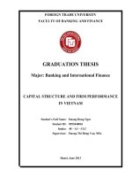
Corporate Valuation and Capital Structure
A firm’s financing choices obviously have a direct effect
on the weighted average cost of capital (WACC). Fi-
nancing choices also have an indirect effect on the
costs of debt and equity because they change the risk
and required returns of debt and equity. Financing

choices can also affect free cash flows if the probability
of bankruptcy becomes high. This chapter focuses on
the debt–equity choice and its effect on value.
Value =
+
…
++
FCF
1
FCF
∞
(1 + WACC)
1
FCF
2
(1 + WACC)
2
(1 + WACC)
∞
Free cash flow
(FCF)
Market interest rates
Firm’s business riskMarket risk aversion
Cost of debt
Cost of equity
Weighted average
cost of capital
(WACC)
Firm’s
debt/equity

mix
Required investments
in operating capital
Net operating
profit after taxes
–
=
resource
The textbook’s Web site
contains an Excel file that
will guide you through the
chapter’s calculations.
The file for this chapter is
Ch15 Tool Kit.xls, and
we encourage you to
open the file and follow
along as you read the
chapter.
600 Part 6: Cash Distributions and Capital Structure
V
op
¼
∑
∞
t¼1
FCF
t
ð1þWACCÞ
t
(15-1)

The WACC depends on the percentages of debt and common equity (w
d
and w
s
),
the cost of debt (r
d
), the cost of stock (r
s
), and the corporate tax rate (T):
WACC = w
d
(1 − T)r
d
+w
s
r
s
(15-2)
As these equations show, the only way any decision can change a firm’svalueis
by affecting either free cash flows or the cost of capital. We discuss below some of
the ways that a higher proportion of debt can affect WACC and/or FCF.
Debt Increases the Cost of Stock, r
s
Debtholders have a claim on the company’s cash flows that is prior to shareholders,
who are entitled only to any residual cash flow after debtholders have been paid.
As we show later in a numerical example, the “fixed” claim of the debtholders causes
the “residual” claim of the stockholders to become riskier, and this increases the cost
of stock, r
s

.
Debt Reduces the Taxes a Company Pays
Imagine that a company’s cash flows are a pie and that three different groups get
pieces of the pie. The first piece goes to the government in the form of taxes, the
second goes to debtholders, and the third to shareholders. Companies can deduct
interest expenses when calculating taxable income, which reduces the government’s
piece of the pie and leaves more pie available to debtholders and investors. This
reduction in taxes reduces the after-tax cost of debt, as shown in Equation 15-2.
The Risk of Bankr uptcy Increases the Cost of Debt, r
d
As debt increases, the probability of financial distress, or even bankruptcy, goes up.
With higher bankruptcy risk, debtholders will insist on a higher interest rate, which
increases the pre-tax cost of debt, r
d
.
The Net Effect on the Weighted Average Cost of Capital
As Equation 15-2 shows, the WACC is a weighted average of relatively low-cost debt
and high-cost equity. If we increase the proportion of debt, then the weight of
low-cost debt (w
d
) increases and the weight of high-cost equity (w
s
) decreases. If all
else remained the same, then the WACC would fall and the value of the firm in
Equation 15-1 would increase. But the previous paragraphs show that all else doesn’t
remain the same: both r
d
and r
s
increase. It should be clear that changing the capital

structure affects all the variables in the WACC equation, but it’s not easy to say
whether those changes increase the WACC, decrease it, or balance out exactly and
thus leave the WACC unchanged. We’ll return to this issue later when discussing
capital structure theory.
Bankruptcy Risk Reduces Free Cash Flow
As the risk of bankruptcy increases, some customers may choose to buy from another
company, which hurts sales. This, in turn, decreases net operating profit after taxes
(NOPAT), thus reducing FCF. Financial distress also hurts the productivity of
Chapter 15: Capital Structure Decisions 601
workers and managers, who spend more time worrying about their next job than
attending to their current job. Again, this reduces NOPAT and FCF. Finally, suppli-
ers tighten their credit standards, which reduces accounts payable and causes net
operating working capital to increase, thus reducing FCF. Therefore, the risk of
bankruptcy can decrease FCF and reduce the value of the firm.
Bankruptcy Risk Affects Agency Costs
Higher levels of debt may affect the behavior of managers in two opposing ways.
First, when times are good, managers may waste cash flow on perquisites and
unnecessary expenditures. This is an agency cost, as described in Chapter 13. The
good news is that the threat of bankruptcy reduces such wasteful spending, which
increases FCF.
But the bad news is that a manager may become gun-shy and reject positive-NPV
projects if they are risky. From the stockholder’s point of view, it would be unfortu-
nate if a risky project caused the company to go into bankruptcy, but note that other
companies in the stockholder’s portfolio may be taking on risky projects that turn out
to be successful. Since most stockholders are well diversified, they can afford for a
manager to take on risky but positive-NPV projects. But a manager’s reputation and
wealth are generally tied to a single company, so the project may be unacceptably
risky from the manager’s point of view. Thus, high debt can cause managers to forgo
positive-NPV projects unless they are extremely safe. This is called the underinvest-
ment problem, and it is another type of agency cost. Notice that debt can reduce

one aspect of agency costs (wasteful spending) but may increase another (underin-
vestment), so the net effect on value isn’t clear.
Issui ng Equity Conveys a Signal to the Market place
Managers are in a better position to forecast a company’s free cash flow than are
investors, and academics call this informational asymmetry. Suppose a company’s
stock price is $50 per share. If managers are willing to issue new stock at $50 per
share, investors reason that no one would sell anything for less than its true value.
Therefore, the true value of the shares as seen by the managers with their superior
information must be less than or equal to $50. Thus, investors perceive an equity
issue as a negative signal, and this usually causes the stock price to fall.
1
In addition to affecting investors’ perceptions, capital structure choices also affect
FCF and risk, as discussed earlier. The following section focuses on the way that
capital structure affects risk.
A Quick Overview of Actual Debt Ratios
For the average company in the S&P 500, the ratio of long-term debt to equity was
about 92% in the summer of 2009. This means that the typical company had about
$0.92 in debt for every dollar of equity. However, Table 15-1 shows that there are
wide divergences in the average ratios for different business sectors and for different
companies within a sector. For example, the technology sector has a very low average
ratio (23%) while the utilities sector has a much higher ratio (177%). Even so, within
each sector there are some companies with low levels of debt and others with high
1
An exception to this rule is any situation with little informational asymmetry, such as a regulated utility.
Also, some companies, such as start-ups or high-tech ventures, are unable to find willing lenders and
therefore must issue equity; we discuss this later in the chapter.
602 Part 6: Cash Distributions and Capital Structure
levels. For example, the average debt ratio for the consumer/noncyclical sector is
38%, but in this sector Starbucks has a ratio of 21% while Kellogg has a ratio of
280%. Why do we see such variation across companies and business sectors? Can a

company make itself more valuable through its choice of debt ratio? We address
those questions in the rest of this chapter, beginning with a description of business
risk and financial risk.
Self-Test
Briefly describe some ways in which the capital structure decision can affect the
WACC and FCF.
15.2 BUSINESS RISK AND FINANCIAL RISK
Business risk and financial risk combine to determine the total risk of a firm’s future
return on equity, as we explained in the next sections.
Business Risk
Business risk is the risk a firm’s common stockholders would face if the firm had no
debt. In other words, it is the risk inherent in the firm’s operations, which arises from
uncertainty about future operating profits and capital requirements.
Business risk depends on a number of factors, beginning with variability in prod-
uct demand. For example, General Motors has more demand variability than does
Kroger: When times are tough, consumers quit buying cars but they still buy food.
Second, most firms are exposed to variability in sales prices and input costs. Some
firms with strong brand identity like Apple may be able to pass unexpected costs
through to their customers, and firms with strong market power like Wal-Mart may
be able to keep their input costs low, but variability in prices and costs adds signifi-
cant risk to most firms’ operations. Third, firms that are slower to bring new
Long-Term Debt-to-Equity Ratios for Selected Firms and Industries
TABLE 15-1
SECTOR AND COMPANY
LONG-TERM
DEBT-TO-
EQUITY RATIO
SECTOR AND
COMPANY
LONG-TERM

DEBT-TO-
EQUITY RATIO
Technology 23% Capital Goods 38%
Microsoft (MSFT) 0 Winnebago Industries (WGO)
0
Ricoh (RICTEYR.Lp) 25 Caterpillar Inc. (CAT) 375
Energy 64 Consumer/Noncyclical 38
ExxonMobil (XOM) 6 Starbucks (SBUX) 21
Chesapeake Energy (CHK) 87 Kellogg Company (K) 280
Transportation 84 Services 84
United Parcel Service (UPS) 115 Administaff, Inc. (ASF) 0
Continental Airlines (CAL) 5,115 Republic Services (RSG) 99
Basic Materials 45 Utilities 177
Anglo American PLC (AAUK) 36 Reliant Energy, Inc. (RRI) 96
Century Aluminum (CENX) 29 CMS Energy (CMS) 227
Source: For updates on a company’s ratio, go to and enter the ticker symbol for a stock quote. Click on Ratios
(on the left) for updates on the sector ratio.
Chapter 15: Capital Structure Decisions 603
products to market have greater business risk: Think of GM’s relatively sluggish time
to bring a new model to the market versus that of Toyota. Being faster to the market
allows Toyota to more quickly respond to changes in consumer desires. Fourth,
international operations add the risk of currency fluctuations and political risk. Fifth,
if a high percentage of a firm’s costs are fixed and hence do not decline when de-
mand falls, then the firm has high operating leverage, which increases its business
risk. We focus on operating leverage in the next section.
Operating Leverage
A high degree of operating leverage implies that a relatively small change in sales
results in a relatively large change in EBIT, net operating profits after taxes (NOPAT),
and return on invested capital (ROIC). Other things held constant, the higher a firm’s
fixed costs, the greater its operating leverage. Higher fixed costs are generally associ-

ated with (1) highly automated, capital intensive firms; (2) businesses that employ
highly skilled workers who must be retained and paid even when sales are low; and
(3) firms with high product development costs that must be maintained to complete
ongoing R&D projects.
To illustrate the relative impact of fixed versus variable costs, consider Strasburg
Electronics Company, a manufacturer of components used in cell phones. Strasburg
is considering several different operating technologies and several different financing
alternatives. We will analyze its financing choices in the next section, but for now we
focus on its operating plans.
Each of Strasburg’s plans requires a capital investment of $200 million; assume for
now that Strasburg will finance its choice entirely with equity.
2
Each plan is expected
to produce 100 million units per year at a sales price of $2 per unit. As shown in
Figure 15-1, Plan A’s technology requires a smaller annual fixed cost than Plan U’s,
but Plan A has higher variable costs. (We denote the second plan with U because it
has no financial leverage, and we denote the third plan with L because it does have
financial leverage; Plan L is discussed in the next section.) Figure 15-1 also shows the
projected income statements and selected performance measures for the first year.
Notice that Plan U has higher net income, higher net operating profit after taxes
(NOPAT), higher return on equity (ROE), and higher return on invested capital
than does Plan A. So at first blush it seems that Strasburg should accept Plan U
instead of Plan A.
Notice that the projections in Figure 15-1 are based on the 110 million units that
are expected to be sold. But what if demand is lower than expected? It often is useful
to know how far sales can fall before operating profits become negative. The
operating break-even point occurs when earnings before interest and taxes (EBIT)
equal zero (P, Q, V, and F are defined in Figure 15-1):
3
EBIT = PQ − VQ − F=0

(15-3)
2
Strasburg has improved its supply chain operations to such an extent that its operating current assets are
not larger than its operating current liabilities. In fact, its Op CA = Op CL = $10 million. Recall that net
operating working capital (NOWC) is the difference between Op CA and Op CL, so Strasburg has
NOWC = 0. Even though Strasburg’s plans require $210 million in assets, they also generate $10 million
in spontaneous operating liabilities, so Strasburg’s investors must put up only $200 million in some
combination of debt and equity.
3
This definition of the break-even point does not include any fixed financial costs because it focuses on
operating profits. We could also examine net income, in which case a levered firm would suffer an
accounting loss even at the operating break-even point. We introduce financial costs shortly.
604 Part 6: Cash Distributions and Capital Structure
If we solve for the break-even quantity, Q
BE
, we get this expression:
Q
BE
¼
F
P − V
(15-4)
The break-even quantities for Plans A and U are
Plan A: Q
BE
¼
$20;000
$2:00 − $1:50
¼ 40;000 units
Plan U: Q

BE
¼
$60;000
$2:00 − $1:00
¼ 60;000 units
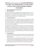
Plan A will be profitable if unit sales are above 40,000, whereas Plan U requires
sales of 60,000 units before it is profitable. This difference is because Plan U has
higher fixed costs, so more units must be sold to cover these fixed costs. Panel a of
Figure 15-2 illustrates the operating profitability of these two plans for different
levels of unit sales. (We discuss Panel b in the next section.) Suppose sales are
at 80 million units. In this case, the NOPAT is identical for each plan. As unit
sales begin to climb above 80 million, both plans increase in profitability, but
FIGURE 15-1
Illustration of Operating and Financial Leverage (Millions of Dollars and Millions of Units,
Except Per Unit Data)
Input Data
Plan A
Plan U
Plan L
Required capital
$200
$200 $200
Book equity
$200
$200 $150
Debt
$50
Interest rate
8%
8%

8%
Sales price (P)
$2.00
$2.00
$2.00
Tax rate (T)
40%
40%
40%
Expected units sold (Q)
110
110
110
Fixed costs (F)
$20
$60
$60
Variable costs (V)
$1.50
$1.00
$1.00
Income Statements
Plan A
Plan U
Plan L
Sales revenue (P×Q)
$220.0
$220.0
$220.0
Fixed costs

$20.0
$60.0
$60.0
Variable costs (V×Q)
$165.0
$110.0
$110.0
EBIT
$35.0
$50.0
$50.0
Interest
$0.0
$0.0
$4.0
EBT
$35.0
$50.0
$46.0
Tax
$14.0
$20.0
$18.4
Net income
$21.0
$30.0
$27.6
Key Performance Measures
Plan A
Plan U Plan L

NOPAT = EBIT(1–T)
$21.0
$30.0
$30.0
ROIC = NOPAT/Capital
10.5%
15.0%
15.0%
ROE = NI/Equity
10.5%
15.0%
18.4%
Chapter 15: Capital Structure Decisions 605
NOPAT increases more for Plan U than for Plan A. If sales fall below 80 million
then both plans become less profitable, but NOPAT decreases more for Plan U
than for Plan A. This illustrates that the combination of higher fixed costs and
lower variable costs of Plan U magni fies its gain or loss relative to Plan A. In
other words, because Plan U has higher operating leverage, it also has greater
business risk.
Notice that business risk is being driven by variability in the number of units
that can be sold. It would be straightforward to estimate a probability for each
possible level of sales and then calculate the standard deviation of the resulting
NOPATs in exactly the same way that we calculated project risk using scenario
analysis in Chapter 11. This would produce a quantitative estimate of business
risk.
4
However, for most purposes it is sufficient to recognize that business risk
increases if operating leverage increases and then use that insight qualitatively
rather than quantitatively when evaluating plans with different degrees of operat-
ing leverage.

FIGURE 15-2 Operating Leverage and Financial Leverage
Panel a: Operating Leverage
Plan A
Plan U
–$50
–
$40
–$30
–$20
–$10
$0
$10
$20
$30
$40
$50
$60
0 20 40 60 80 100 120 140
Units Sold
(Millions)
NOPAT
(Millions)
Plan U
Break-even Q
Plan A
Break-even Q
Cross Over at
80 Million
Panel b: Financial Leverage
Plan U

Plan L
-6%
0%
6%
12%
18%
0%
6% 12% 18%
Return on
Invested Capital
Return
on Equity
Cross Over at
ROIC = (1−T) × r
d
= 4.8%
4
For this example, we could also directly express the standard deviation of NOPAT, σ
NOPAT
, in terms of
the standard deviation of unit sales, σ
Q
: σ
NOPAT
=(P− V)(1 − T) × σ
Q
. We could also express the standard
deviation of ROIC as σ
ROIC
= [(P − V)(1 − T)/Capital] × σ

Q
. As this shows, volatility in NOPAT (and
ROIC) is driven by volatility in unit sales, with a bigger spread between price and variable costs leading
to higher volatility. Also, there are several other ways to calculate measures of operating leverage, as we
explain in Web Extension 15A.
606 Part 6: Cash Distributions and Capital Structure
Financial Risk
Financial risk is the additional risk placed on the common stockholders as a result of
the decision to finance with debt.
5
Conceptually, stockholders face a certain amount of
risk that is inherent in a firm’s operations—this is its business risk, which is defined as
the uncertainty in projections of future EBIT, NOPAT, and ROIC. If a firm uses debt
(financial leverage), then the business risk is concentrated on the common stockholders.
To illustra te, suppose ten people decide to form a corporation to manufacture flash
memory drives. There is a certain amount of business risk in the operation. If the firm
is capitalized only with common equity and if each person buys 10% of the stock, then
each investor shares equally in the business risk. However, suppose the firm is capital-
ized with 50% debt and 50% equity, with five of the investors putting up their money
by purchasing debt and the other five putting up their money by purchasing equity. In
this case, the five debtholders are paid before the five stockholders, so virtually all of the
business risk is borne by the stockholders. Thus, the use of debt, or financial leverage,
concentrates business risk on stockholders.
6
To illustrate the impact of financial risk, we can extend the Strasburg Electronics
example. Strasburg initially decided to use the technology of Plan U, which is unlev-
ered (financed with all equity), but now it’s considering financing the technology
with $150 million of equity and $50 million of debt at an 8% interest rate, as shown
for Plan L in Figure 15-1 (recall that L denotes leverage). Compare Plans U and L.
Notice that the ROIC of 15% is the same for the two plans because the financing

choice doesn’t affect operations. Plan L has lower net income ($27.6 million versus
$30 million) because it must pay interest, but it has a higher ROE (18.4%) because
the net income is shared over a smaller equity base.
7
Suppose Strasburg is a zero-growth company and pays out all net income as
dividends. This means that Plan U has net income of $30 million available for
distribution to its investors. Plan L has $27.6 million net income available to pay
as dividends and it already pays $4 million in interest to its debtholders, so its total
distribution is $27.6 + $4 = $31.6 million. How is it that Plan L is able to distribute
a larger total amount to investors? Look closely at the t axes paid under the two
plans. Plan L pays only $18.4 million in tax while Plan U pays $20 million. The
$1.6 million difference is because interest payments are deductible for tax purposes.
Because Plan L pays less in taxes, an extra $1.6 million is available to distribute to
investors. If our analysis ended here, we would choose Plan L over Plan U because
Plan L distributes more cash to investors and provides a higher ROE for its equity
holders.
But there is more to the story. Just as operating leverage adds risk, so does finan-
cial leverage. We used the Data Table feature in the file Ch15 Tool Kit.xls to gener-
ate performance measures for plans U and L at different levels of unit sales, which
lead to different levels of ROIC. Panel b of Figure 15-2 shows the ROE of Plan L
versus its ROIC. (Keep in mind that the ROIC for Plan U is the same as for Plan L
because leverage doesn’t affect operating performance; also, Plan U’s ROE is the
same as its ROIC because it has no leverage.)
5
Preferred stock also adds to financial risk. To simplify matters, we examine only debt and common
equity in this chapter.
6
Holders of corporate debt generally do bear some business risk, because they may lose some of their
investment if the firm goes bankrupt. We discuss this in more depth later in the chapter.
7

Recall that Strasburg’s operating CA are equal to its operating CL. Strasburg has no short-term
investments, so its book values of debt and equity must sum up to the amount of operating capital it
uses.
Chapter 15: Capital Structure Decisions 607
Notice that for an ROIC of 4.8%, which is the after-tax cost of debt, Plan U
(with no leverage) and Plan L (with leverage) have the same ROE. As ROIC
increases above 6%, the ROE increases for each plan, but more for Plan L than
for Plan U. However, if ROIC falls below 6%, then the ROE falls further for
Plan L than for Plan U. Thus, financial leverage magnifies the ROE for good or
ill, depending on the ROIC, and so increases the risk of a levered firm relative to
an unlevered firm.
8
We see, then, that using leverage has both good and bad effects: If expected
ROIC is greater than the after-tax cost of debt, then higher leverage increases
expected ROE but also increases risk.
Strasburg’s Valuatio n Analysis
Strasburg decided to go with Plan L, the one with high operating leverage and $50
million in debt financing. This resulted in a stock price of $20 per share. With 10
million shares, Strasburg’s market value of equity is $20(10) = $200 million. Strasburg
has no short-term investments, so Strasburg’s total enterprise value is the sum of its
debt and equity: V = $50 + $200 = $250 million. Notice that this is greater than the
required investment, which means that the plan has a positive NPV; another way to
view this is that Strasburg’s Market Value Added (MVA) is positive. In terms of
market values, Strasburg’s capital structure has 20% debt (w
d
= $50/$250 = 0.20) and
80% equity (w
s
= $200/$250 = 0.80). These calculations are reported in Figure 15-3.
Is this the optimal capital structure? We will address the question in more detail

later, but for now let’s focus on understanding Strasburg’s current valuation, begin-
ning with its cost of capital. Strasburg has a beta of 1.25. We can use the Capital
Asset Pricing Model (CAPM) to estimate the cost of equity. The risk-free rate, r
RF
,
is 6.3% and the market risk premium, RP
M
, is 6%, so the cost of equity is
r
s
=r
RF
+ b(RP
M
) = 6.3% + 1.25(6%) = 13.8%
The weighted average cost of capital is
WACC ¼ w
d
ð1 − TÞr
d
þ w
s
r
s
¼ 20%ð1 − 0:40Þð8%Þþ80%ð13:8%Þ
¼ 12%
As shown in Figure 15-1, Plan L has a NOPAT of $30 million. Strasburg
expects zero growth, which means there are no required investments in capital.
Therefore, FCF is equal to NOPAT. Using the constant growth formula, the value
of operations is

V
op
¼
FCFð1 þgÞ
WACC − g
¼
$30ð1 þ 0Þ
0:12 − 0
¼ $250
Figure 15-3 illustrates the calculation of the intrinsic stock price. For Strasburg,
the intrinsic stock price and the market price are each equal to $20. Can Strasburg
increase its value by changing its capital structure? The next section discusses how
the trade-off between risk and return affects the value of the firm, and Section 15.5
estimates the optimal capital structure for Strasburg.
8
We could also express the standard deviation of ROE, σ
ROE
, in terms of the standard deviation
of ROIC: σ
ROE
= (Capital/Equity) × σ
ROIC
= (Capital/Equity) × [(P − V)(1 − T)/Capital]× σ
Q
. Thus,
volatility in ROE is due to the amount of financial leverage, the amount of operating leverage, and the
underlying risk in units sold. This is similar in spirit to the Du Pont model discussed in Chapter 3.
608 Part 6: Cash Distributions and Capital Structure
Self-Test
What is business risk, and how can it be measured?

What are some determinants of business risk?
How does operating leverage affect business risk?
What is financial risk, and how does it arise?
Explain this statement: “Using leverage has both good and bad effects.”
A firm has fixed operating costs of $100,000 and variable costs of $4 per unit. If it
sells the product for $6 per unit, what is the break-even quantity? (50,000)
15.3 CAPITAL STRUCTURE THEORY
In the previous section, we showed how capital structure choices affect a firm’s ROE
and its risk. For a number of reasons, we would expect capital structures to vary
considerably across industries. For example, pharmaceutical companies generally have
very different capital structures than airline companies. Moreover, capital structures
vary among firms within a given industry. What factors explain these differences? In
FIGURE 15-3 Strasburg’s Valuation Analysis (Millions of Dollars Except Per Share Data)
Input Data (Millions Except Per Share Data)
Tax rate
40.00%
Debt (D)
$50.00
Number of shares (n)
10.00
Stock price per share (P)
$20.00
NOPAT
$30.00
Free Cash Flow (FCF)
$30.00
Growth rate in FCF
0.00%
Capital Structure (Millions Except Per Share Data)
Market value of equity (S = P × n)

$200.00
Total value (V = D + S)
$250.00
Percent financed with debt (w
d
= D/V)
20%
Percent financed with stock (w
s
= S/V)
80%
Cost of Capital
Cost of debt (r
d
) 8.00%
Beta (b) 1.25
Risk-free rate (r
RF
) 6.30%
Market risk premium (RP
M
) 6.00%
Cost of equity (r
s
= r
RF
+ b × RP
M
)
13.80%

WACC
12.00%
Intrinsic Valuation (Millions Except Per Share Data)
$250.00
+ Value of ST investments
$0.00
Total intrinsic value of firm
$250.00
− Debt
$50.00
Intrinsic value of equity
$200.00
÷ Number of shares
10.00
Intrinsic price per share
$20.00
Value of operations:
V
op
= [FCF(1+g)]/(WACC–g)
Chapter 15: Capital Structure Decisions 609
an attempt to answer this question, academics and practitioners have developed a num-
ber of theories, and the theories have been subjected to many empirical tests. The
following sections examine several of these theories.
9
Modigliani and Miller: No Taxes
Modern capital structure theory began in 1958, when Professors Franco Modigliani
and Merton Miller (hereafter MM) published what has been called the most influen-
tial finance article ever written.
10

MM’s study was based on some strong assumptions,
which included the following:
1. There are no brokerage costs.
2. There are no taxes.
3. There are no bankruptcy costs.
4. Investors can borrow at the same rate as corporations.
5. All investors have the same information as management about the firm’s future
investment opportunities.
6. EBIT is not affected by the use of debt.
Modigliani and Miller imagined two hypothetical portfolios. The first contains all the
equity of an unlevered firm, so the portfolio’s value is V
U
, the value of an unlevered firm.
Because the firm has no growth (which means it does not need to invest in any new net
assets) and because it pays no taxes, the firm can pay out all of its EBIT in the form of
dividends. Therefore, the cash flow from owning this first portfolio is equal to EBIT.
Now consider a second firm that is identical to the unlevered firm except that it is
partially financed with debt. Th e second portfolio contains all of the lever ed firm’sstock
(S
L
) and debt (D), so the portfolio’s value is V
L
, the total value of the levered firm. If
theinterestrateisr
d
, then the levered firm pays out interest in the amount r
d
D.
Because th e firm is not growing and pays no taxes, it can pay out dividends in the
amount EBIT − r

d
D. If you owned all of the firm’s debt and equity, your cash flow
would be equal to the sum of the interest and dividends: r
d
D + (EBIT − r
d
D) = EBIT.
Therefore, the cash flow from owning this second portfolio is equal to EBIT.
Notice that the cash flow of each portfolio is equal to EBIT. Thus, MM con-
cluded that two portfolios producing the same cash flows must have the same value:
11
V
L
=V
U
=S
L
+D
(15-5)
9
For additional discussion of capital structure theories, see John C. Easterwood and Palani-Rajan Kada-
pakkam, “The Role of Private and Public Debt in Corporate Capital Structures,” Financial Management,
Autumn 1991, pp. 49–57; Gerald T. Garvey, “Leveraging the Underinvestment Problem: How High
Debt and Management Shareholdings Solve the Agency Costs of Free Cash Flow,” Journal of Financial
Research, Summer 1992, pp. 149–166; Milton Harris and Artur Raviv, “Capital Structure and the Informa-
tional Role of Debt,” Journal of Finance, June 1990, pp. 321–349; and Ronen Israel, “Capital Structure and
the Market for Corporate Control: The Defensive Role of Debt Financing,” Journal of Finance, September
1991, pp. 1391–1409.
10
Franco Modigliani and Merton H. Miller, “The Cost of Capital, Corporation Finance, and the Theory

of Investment,” American Economic Review, June 1958, pp. 261–297. Modigliani and Miller each won a
Nobel Prize for their work.
11
They actually showed that if the values of the two portfolios differed, then an investor could engage in
riskless arbitrage: The investor could create a trading strategy (buying one portfolio and selling the other)
that had no risk, required none of the investor’s own cash, and resulted in a positive cash flow for the
investor. This would be such a desirable strategy that everyone would try to implement it. But if everyone
tries to buy the same portfolio, its price will be driven up by market demand, and if everyone tries to sell
a portfolio, its price will be driven down. The net result of the trading activity would be to change the
portfolio’s values until they were equal and no more arbitrage was possible.
610 Part 6: Cash Distributions and Capital Structure
Given their assumptions, MM proved that a firm’s value is unaffected by its capital
structure.
Recall that the WACC is a combination of the cost of debt and the relatively
higher cost of equity, r
s
. As leverage increases, more weight is given to low-cost
debt but equity becomes riskier, which drives up r
s
. Under MM’s assumptions, r
s
increases by exactly enough to keep the WACC constant. Put another way: If MM’s
assumptions are correct, then it doesn’t matter how a firm finances its operations and
so capital structure decisions are irrelevant.
Even though some of their assumptions are obviously unrealistic, MM’s irrele-
vance result is extremely important. By indicating the conditions under which capital
structure is irrelevant, MM also provided us with clues about what is required for
capital structure to be relevant and hence to affect a firm’s value. The work of MM
marked the beginning of modern capital structure research, and subsequent research
has focused on relaxing the MM assumptions in order to develop a more realistic

theory of capital structure.
Modigliani and Miller’s thought process was just as important as their conclusion.
It seems simple now, but their idea that two portfolios with identical cash flows must
also have identical values changed the entire financial world because it led to the
development of options and derivatives. It is no surprise that Modigliani and Miller
received Nobel awards for their work.
Modigliani and Miller II: The Effect of Corporate Taxes
In 1963, MM published a follow-up paper in which they relaxed the assumption that
there are no corporate taxes.
12
The Tax Code allows corporations to deduct interest
payments as an expense, but dividend payments to stockholders are not deductible.
The differential treatment encourages corporations to use debt in their capital struc-
tures. This means that interest payments reduce the taxes paid by a corporation, and
if a corporation pays less to the government then more of its cash flow is available for
its investors. In other words, the tax deductibility of the interest payments shields the
firm’s pre-tax income.
Yogi Berra on the MM Proposition
When a w aitress asked Yogi Berra (Baseball Hall of Fame
catcher for the New York Yankees) whether he wanted
his pizza cut into four pieces or eight, Yogi replied:
“Better make it fou r. I do n’t th ink I c an eat eig ht.”
a
Yogi’s quip helps convey the basic insight of Modigliani
and Miller. The firm’s choice of leverage “slices” the distri-
bution of future cash flows in a way that is like slicing a
pizza. MM recognized that holding a company’s invest-
ment activities fixed is like fixing the size of the pizza; no
information costs means that everyone sees the same
pizza; no taxes means the IRS gets none of the pie; and

no “contracting costs” means nothing sticks to the knife.
So, just as the substance of Yogi’s meal is unaf-
fected by whether the pizza is sliced into four pieces or
eight, the economic substance of the firm is unaffected
by whether the liability side of the balance sheet is
sliced to include more or less debt—at least under the
MM assumptions.
a
Lee Green, Sportswit (New York: Fawcett Crest, 1984), p. 228.
Source: “Yogi Berra on the MM Proposition,” Journal of
Applied Corporate Finance, Winter 1995, p. 6. Reprinted by
permission of Stern Stewart Management.
12
Franco Modigliani and Merton H. Miller, “Corporate Income Taxes and the Cost of Capital:
A Correction,” American Economic Review, June 1963, pp. 433–443.
Chapter 15: Capital Structure Decisions 611
As in their earlier paper, MM introduced a second important way of looking at the
effect of capital structure: The value of a levered firm is the value of an otherwise
identical unlevered firm plus the value of any “side effects.” While others have
expanded on this idea by considering other side effects, MM focused on the tax
shield:
V
L
=V
U
+ Value of side effects = V
U
+ PV of tax shield
(15-6)
Under their assumptions, they showed that the present value of the tax shield is equal

to the corporate tax rate, T, multiplied by the amount of debt, D:
V
L
=V
U
+TD
(15-7)
With a tax rate of about 40%, this implies that every dollar of debt adds about 40
cents of value to the firm, and this leads to the conclusion that the optimal capital
structure is virtually 100% debt. MM also showed that the cost of equity, r
s
,
increases as leverage increases but that it doesn’t increase quite as fast as it would
if there were no taxes. As a result, under MM with corporate taxes the WACC falls
as debt is added.
Miller: The Effect of Corporate and Personal Taxes
Merton Miller (this time without Modigliani) later brought in the effects of
personal taxes.
13
The income from bonds is generally interest, which is taxed as
personal income at rates (T
d
) going up to 35%, while income from stocks generally
comes partly from dividends and partly from capital gains. Long-term capital gains
are taxed at a rate of 15%, and this tax is deferred until the stock is sold and the
gain realized. If stock is held until the owner dies, no capital gains tax whatsoever
must be paid. So, on average, returns on stocks are taxed at lower effective rates
(T
s
) than returns on debt.

14
Because of the t ax s ituation, Miller arg ued that i nvestors are wil ling to acce p t
relatively low before-tax returns on stock relative to the before-tax returns on bonds.
(The situation here is similar to that with tax-exempt municipal bonds as discussed in
Chapter 5 and preferred stocks held by corporate investors as discussed in Chapter 7.)
For example, an investor might require a return of 10% on Strasburg’s bonds, and if
stock income were taxed at the same rate as bond income, the required rate of return
on Strasburg’s stock might be 16% because of the stock’s greater risk. H owever, in
view of the favorable treatment of income on the stock, investors might be willing to ac-
cept a before-tax return of only 14% on the stock.
Thus, as Miller pointed out, (1) the deductibility of interest favors the use of debt
financing, but (2) the more favorable tax treatment of income from stock lowers the
required rate of return on stock and thus favors the use of equity financing.
Miller showed that the net impact of corporate and personal taxes is given by this
equation:
13
See Merton H. Miller, “Debt and Taxes,” Journal of Finance, May 1977, pp. 261–275.
14
The Tax Code isn’t quite as simple as this. An increasing number of investors face the Alternative
Minimum Tax (AMT); see Web Extension 2A for a discussion. The AMT imposes a 28% tax rate on
most income and an effective rate of 22% on long-term capital gains and dividends. Under the AMT
there is still a spread between the tax rates on interest income and stock income, but the spread is nar-
rower. See Leonard Burman, William Gale, Greg Leiserson, and Jeffrey Rohaly, “The AMT: What’s
Wrong and How to Fix It,” National Tax Journal, September 2007, pp. 385–405.
612 Part 6: Cash Distributions and Capital Structure
V
L
¼ V
U
þ 1−

ð1 − T
c
Þð1 − T
s
Þ
ð1 − T
d
Þ
!
D
(15-8)
Here T
c
is the corporate tax rate, T
s
is the personal tax rate on income from stocks,
and T
d
is the tax rate on income from debt. Miller argued that the marginal tax rates
on stock and debt balance out in such a way that the bracketed term in Equation 15-8
is zero and so V
L
=V
U
, but most observers believe there is still a tax advantage to debt
if reasonable values of tax rates are assumed. For example, if the marginal corporate tax
rate is 40%, the marginal rate on debt is 30%, and the marginal rate on stock is 12%,
then the advantage of debt financing is
V
L

¼ V
U
þ 1−
ð1 − 0:40Þð1 − 0:12Þ
ð1 − 0:30Þ
!
¼ V
U
þ 0:25D
D
(15-8a)
Thus it appears that the presence of personal taxes reduces but does not completely
eliminate the advantage of debt financing.
Trade-off Theory
The results of Modigliani and Miller also depend on the assumption that there are
no bankruptcy costs. However, bankruptcy can be quite costly. Firms in bankruptcy
have very high legal and accounting expenses, and they also have a hard time retain-
ing customers, suppliers, and employees. Moreover, bankruptcy often forces a firm to
liquidate or sell assets for less than they would be worth if the firm were to continue
operating. For example, if a steel manufacturer goes out of business it might be hard
to find buyers for the company’ s blast furnaces. Such assets are often illiquid because
they are configured to a company’s individual needs and also because they are
difficult to disassemble and move.
Note, too, that the threat of bankruptcy, not just bankruptcy per se, causes many of
these same problems. Key employees jump ship, suppliers refuse to grant credit,
customers seek more stable suppliers, and lenders demand higher interest rates and
impose more restrictive loan covenants if potential bankruptcy looms.
Bankruptcy-related problems are most likely to arise when a firm includes a great
deal of debt in its capital structure. Therefore, bankruptcy costs discourage firms
from pushing their use of debt to excessive levels.

Bankruptcy-related costs have two components: (1) the probability of financial
distress and (2) the costs that would be incurred if financial distress does occur. Firms
whose earnings are more volatile, all else equal, face a greater chance of bankruptcy
and should therefore use less debt than more stable firms. This is consistent with our
earlier point that firms with high operating leverage, and thus greater business risk,
should limit their use of financial leverage. Likewise, firms that would face high costs
in the event of financial distress should rely less heavily on debt. For example, firms
whose assets are illiquid and thus would have to be sold at “ fire sale” prices should
limit their use of debt financing.
The preceding arguments led to the development of what is called the trade-off
theory of leverage, in which firms trade off the benefits of debt financing (favorable
corporate tax treatment) against higher interest rates and bankruptcy costs. In
essence, the trade-off theory says that the value of a levered firm is equal to the
Chapter 15: Capital Structure Decisions 613
value of an unlevered firm plus the value of any side effects, which include the tax
shield and the expected costs due to financial distress. A summary of the trade-off
theory is expressed graphically in Figure 15-4, and a list of observations about the
figure follows here.
1. Under the assumptions of the MM model with corporate taxes, a firm’s value
increases linearly for every dollar of debt. The line labeled “MM Result Incor-
porating the Effects of Corporate Taxation” in Figure 15-4 expresses the rela-
tionship between value and debt under those assumptions.
2. There is some threshold level of debt, labeled D
1
in Figure 15-4, below which
the probability of bankruptcy is so low as to be immaterial. Beyond D
1
, however,
expected bankruptcy-related costs become increasingly important, and they
reduce the tax benefits of debt at an increasing rate. In the range from D

1
to D
2
,
expected bankruptcy-related costs reduce but do not completely offset the tax
benefits of debt, so the stock price rises (but at a decreasing rate) as the debt ratio
increases. However, beyond D
2
, expected bankruptcy-related costs exceed the
tax benefits, so from this point on increasing the debt ratio lowers the value of
the stock. Therefore, D
2
is the optimal capital structure. Of course, D
1
and D
2
vary from firm to firm, depending on their business risks and bankruptcy costs.
3. Although theoretical and empirical work confirm the general shape of the curve
in Figure 15-4, this graph must be taken as an approximation and not as a
precisely defined function.
Signaling Theory
It was assumed by MM that inve stors have the same information about a firm’s prospects
as its managers—this is called symmetric information. However, managers i n fact often
have better information than outside investors. This is called asymmetric information ,
FIGURE 15-4 Effect of Financial Leverage on Value
Value
Value Added by
Debt Tax Shelter
Benets
MM Result Incorporating the

Effects of Corporate Taxation:
Value If There Were No
Bankruptcy-Related Costs
Value Reduced by
Bankruptcy-Related Costs
Actual Value
Value If the Firm
Used No Financial
Leverage
Leverage0DD
12
Value with
Zero Debt
Threshold Debt Level
Where Bankruptcy
Costs Become Material
Optimal Capital Structure:
Marginal Tax Shelter Benets =
Mar
g
inal Bankruptcy-Related Costs
614 Part 6: Cash Distributions and Capital Structure
and it has a n important effect on the optimal capital structure. To see why, consider two
situations, one in which the company’s managers know that its prospects are extremely
positive (Firm P) and one in which the managers know that the future l ooks negative
(Firm N).
Suppose, for example, that Firm P’s R&D labs have just discovered a nonpatentable
cure for the common cold. They want to keep the new product a secret as long as
possible to delay competitors’ entry into the market. New plants must be built to
make the new product, so capital must be raised. How should Firm P’s management

raise the needed capital? If it sells stock then, when profits from the new product start
flowing in, the price of the stock would rise sharply and the purchasers of the new
stock would make a bonanza. The current stockholders (including the managers) would
also do well, but not as well as they would have done if the company had not sold stock
before the price increased, because then they would not have had to share the benefits
of the new product with the new stockholders. Therefore, we should expect a firm with
very positive prospects to avoid selling stock and instead to raise required new capital by other
means, including debt usage beyond the normal target capital structure.
15
Now let’s consider Firm N. Suppose its managers have information that new orders
are off sharply because a competitor has installed new technology that has improved its
products’ quality. Firm N must upgrade its own facilities, at a high cost, just to maintain
its current sales. As a result, its return o n investment will fall (but not by as much as if it
took no action, which would lead to a 100% lo ss through bankruptcy). How should Firm
N raise the needed capital? Here the situation is just the reverse of that facing Firm P,
which did not want to sell stock so as to avoid having to share the benefits of future devel-
opments. A firm with negative prospects would want to sell stock, which would mean bringing
in new investors to share the losses!
16
The conclusion from all this is that firms with ex-
tremely bright prospects prefer not to finance through new stock offerings, whereas firms
with poor prospects like to finance with outside equity. How should you, as an investor,
react to this conclusion? You ought to say: “If I see that a company plans to issue new
stock, this should worry me b ecause I know that management would not want to issue
stock if future prospects looked good. However, management would want to issue stock
if things looked bad. Theref ore, I should lower my estimate of the firm’svalue,other
things held constant, if it plans to issue new stock.”
If you gave this answer then your views are consistent with those of sophisticated
portfolio managers. In a nutshell: The announcement of a stock offering is generally taken
as a signal that the firm’s prospects as seen by its own management are not good; conversely,

a debt offering is taken as a positive signal. Notice that Firm N’s managers cannot make
a false signal to investors by mimicking Firm P and issuing debt. With its unfavorable
future prospects, issuing debt could soon force Firm N into bankruptcy. Given the
resulting damage to the personal wealth and reputations of N’s managers, they can-
not afford to mimic Firm P. All of this suggests that when a firm announces a new
stock offering, more often than not the price of its stock will decline. Empirical stud-
ies have shown that this is indeed true.
Reserve Borrowing Capacity
Because issuing stock sends a negative signal and tends to depress the stock price even if
the company’s true prospects are bright, a company should try to maintain a reserve
15
It would be illegal for Firm P’s managers to personally purchase more shares on the basis of their inside
knowledge of the new product.
16
Of course, Firm N would have to make certain disclosures when it offered new shares to the public, but
it might be able to meet the legal requirements without fully disclosing management’s worst fears.
Chapter 15: Capital Structure Decisions 615
borrowing capacity so that debt can be used if an especially good investment opportunity
comes along. This means that firms should, in normal times, use more equity and less debt than
is suggested by the tax benefit –bankruptcy c ost trade-off model depicted in Fi gure 15-4.
The Pecking Order Hypothesis
The presence of flotation costs and asymmetric information may cause a firm to raise
capital according to a pecking order. In this situation, a firm first raises capital inter-
nally by reinvesting its net income and selling its short-term marketable securities.
When that supply of funds has been exhausted, the firm will issue debt and perhaps
preferred stock. Only as a last resort will the firm issue common stock.
17
Usin g Debt Financi ng to Constrain Managers
Agency problems may arise if managers and shareholders have different objectives.
Such conflicts are particularly likely when the firm’s managers have too much cash

at their disposal. Managers often use excess cash to finance pet projects or for perqui-
sites such as nicer offices, corporate jets, and sky boxes at sports arenas—none of
which have much to do with maximizing stock prices. Even worse, managers might
be tempted to pay too much for an acquisition, something that could cost share-
holders hundreds of millions of dollars. By contrast, managers with limited “excess
cash flow” are less able to make wasteful expenditures.
Firms can reduce excess cash flow in a variety of ways. One way is to funnel some
of it back to shareholders through higher dividends or stock repurchases. Another
alternative is to shift the capital structure toward more debt in the hope that higher
debt service requirements will force managers to be more disciplined. If debt is not
serviced as required then the firm will be forced into bankruptcy, in which case its
managers would likely lose their jobs. Therefore, a manager is less likely to buy an
expensive new corporate jet if the firm has large debt service requirements that could
cost the manager his or her job. In short, high levels of debt bond the cash flow,
since much of it is precommitted to servicing the debt.
A leveraged buyout (LBO) is one way to bond cash flow. In an LBO, a large amount
of debt and a small amount of cash are used to finance the purchase of a company’sshares,
after which the firm “goes private.” The f irst wave of LBOs was i n the mid-1980s; private
equity funds led the buyouts of the late 1990s and early 2000s. Many of these LBOs were
specifically designed to reduce corporate waste. As noted, high debt payments force
managers to conserve cash by eliminating unnecessary expenditures.
Of course, increasing debt and reducing the available cash flow has its downside: It
increases the risk of bankruptcy. Ben Bernanke, current (summer 2009) chairman of
the Fed, has argued that adding debt to a firm’s capital structure is like putting a
dagger into the steering wheel of a car.
18
The dagger—which points toward your
stomach—motivates you to drive more carefully, but you may get stabbed if someone
runs into you—even if you are being careful. The analogy applies to corporations in
the following sense: Higher debt forces managers to be more careful with share-

holders’ money, but even well-run firms could face bankruptcy (get stabbed) if some
event beyond their control occurs: a war, an earthquake, a strike, or a recession. To
complete the analogy, the capital structure decision comes down to deciding how
long a dagger stockholders should use to keep managers in line.
17
For more information, see Jonathon Baskin, “An Empirical Investigation of the Pecking Order
Hypothesis,” Financial Management, Spring 1989, pp. 26–35.
18
See Ben Bernanke, “Is There Too Much Corporate Debt?” Federal Reserve Bank of Philadelphia Business
Review, September/October 1989, pp. 3–13.
616 Part 6: Cash Distributions and Capital Structure
Finally, too much debt may overconstrain managers. A large portion of a man-
ager’s personal wealth and reputation is tied to a single company, so managers are
not well diversified. When faced with a positive-NPV project that is risky, a manager
may decide that it’s not worth taking on the risk even though well-diversified stock-
holders would find the risk acceptable. As previously mentioned, this is an underin-
vestment problem. The more debt the firm has, the greater the likelihood of financial
distress and thus the greater the likelihood that managers will forgo risky projects
even if they have positive NPVs.
The Investment Opportunity Set and Reserve
Borrowing Capacity
Bankruptcy and financial distress are costly, and, as just reiterated, this can discourage
highly levered firms from undertaking risky new investments. If potential new invest-
ments, although risky, have positive net present values, then high levels of debt can be
doubly costly—the expected finan cial distress and bankruptcy costs are high, and
the firm loses potential value by not making some potentially profitable investments. On
the o ther hand, if a firm has very few profitab le investment opportunities then high levels
of debt can keep managers from wasting money by investing in poor projects. For such
companies, increases in the debt ratio can actua lly increase the value of the firm.
Thus, in addition to the tax, signaling, bankruptcy, and managerial constraint ef-

fects discussed previously, the firm’s optimal capital structure is related to its set of
investment opportunities. Firms with many profitable opportunities should maintain
their ability to invest by using low levels of debt, which is also consistent with main-
taining reserve borrowing capacity. Firms with few profitable investment opportu-
nities should use high levels of debt (which have high interest payments) to impose
managerial constraint.
19
Windows of Opportunity
If markets are efficient, then security prices should reflect all available informa-
tion; hence they are neither underpriced nor overpriced (except during the time
it takes prices to move to a new equilibrium caused by the release of new infor-
mation). The windows of opportunity theory states that managers don’t believe this
and supposes instead that stock prices and interest rates are sometimes either too
low or too high relative to their true fundamental values. In particular, the theory
suggests that managers issue equity when they believe stock market prices are
abnormally high and issue debt when they believe interest rates are abnormally
low. In other words, they try to time the market.
20
Notice that this differs from
signaling theory because no asymmetric information is involved: These managers
aren’t basing their beliefs on insider information, just on a difference of opinion
with the market consensus.
Self-Test
Why does the MM theory with corporate taxes lead to 100% debt?
Explain how asymmetric information and signals affect capital structure decisions.
What is meant by reserve borrowing capacity, and why is it important to firms?
How can the use of debt serve to discipline managers?
19
See Michael J. Barclay and Clifford W. Smith, Jr., “The Capital Structure Puzzle: Another Look at the
Evidence,” Journal of Applied Corporate Finance, Spring 1999, pp. 8–20.

20
See Malcolm Baker and Jeffrey Wurgler, “Market Timing and Capital Structure,” Journal of Finance,
February 2002, pp. 1–32.
Chapter 15: Capital Structure Decisions 617
15.4 CAPITAL STRUCTURE EVIDENCE AND IMPLICATIONS
There have been hundreds, perhaps even thousands, of papers testing the capital
structure theories described in the previous section. We can cover only the highlights
here, beginning with the empirical evidence.
21
Empirical Evidence
Studies show that firms do benefit from the tax deductibility of interest payments,
with a typical firm increasing in value by about $0.10 for every dollar of debt. This
is much less than the corporate tax rate, which supports the Miller model (with
corporate and personal taxes) more than the MM model (with only corporate taxes).
Recent evidence shows that the cost of bankruptcies can be as much as 10% to 20%
of the firm’s value.
22
Thus, the evidence shows the existence of tax benefits and
financial distress costs, which provides support for the trade-off theory.
A particularly interesting study by Professors Mehotra, Mikkelson, and Partch ex-
amined the capital structure of firms that were spun off from their parents.
23
The
financing choices of existing firms might be influenced by their past financing choices
and by the costs of moving from one capital structure to another, but because spin-
offs are newly created companies, managers can choose a capital structure without
regard to these issues. The study found that more profitable firms (which have a
lower expected probability of bankruptcy) and more asset-intensive firms (which
have better collateral and thus a lower cost of bankruptcy should one occur) have
higher levels of debt. These findings support the trade-off theory.

However, there is also evidence that is inconsistent with the static optimal target
capital structure implied by the trade-off theory. For example, stock prices are
volatile, which frequently causes a firm’s actual market-based debt ratio to deviate
from its target. However, such deviations don’t cause firms to immediately return to
their target by issuing or repurchasing securities. Instead, firms tend to make a partial
adjustment each year, moving about one-third of the way toward their target capital
structure.
24
This evidence supports the idea of a more dynamic trade-off theory
in which firms have target capital structures but don’t strive to maintain them
too closely.
If a stock price has a big run-up, which reduces the debt ratio, then the trade-off
theory suggests that the firm should issue debt to return to its target. However, firms
tend to do the opposite, issuing stock after big run-ups. This is much more consistent
with the windows of opportunity theory, with managers trying to time the market by
issuing stock when they perceive the market to be overvalued. Furthermore, firms
tend to issue debt when stock prices and interest rates are low. The maturity of the
issued debt seems to reflect an attempt to time interest rates: Firms tend to issue
short-term debt if the term structure is upward sloping but long-term debt if the
21
This section also draws heavily from Barclay and Smith, “The Capital Structure Puzzle,” cited in
footnote 19; Jay Ritter, ed., Recent Developments in Corporate Finance (Northampton, MA: Edward Elgar
Publishing Inc., 2005); and a presentation by Jay Ritter at the 2003 FMA meeting, “The Windows of
Opportunity Theory of Capital Structure.”
22
The expected cost of financial distress is the product of bankruptcy costs and the probability of
bankruptcy. At moderate levels of debt with low probabilities of bankruptcy, the expected cost of financial
distress would be much less than the actual bankruptcy costs if the firm failed.
23
See V. Mehotra, W. Mikkelson, and M. Partch, “The Design of Financial Policies in Corporate Spin-

offs,” Review of Financial Studies, Winter 2003, pp. 1359–1388.
24
See Mark Flannery and Kasturi Rangan, “Partial Adjustment toward Target Capital Structures,” Journal
of Financial Economics, Vol. 79, 2006, pp. 469–506.
618 Part 6: Cash Distributions and Capital Structure
term structure is flat. Again, these facts suggest that managers try to time the market,
which is consistent with the windows of opportunity theory.
Firms issue equity much less frequently than debt. On the surface, this seems to
support both the pecking order hypothesis and the signaling hypothesis. The pecking
order hypothesis predicts that firms with a high level of informational asymmetry,
which causes equity issuances to be costly, should issue debt before issuing equity.
Yet we often see the opposite, with high-growth firms (which usually have greater
informational asymmetry) issuing more equity than debt. Also, many highly profit-
able firms could afford to issue debt (which comes before equity in the pecking
order) but instead choose to issue equity. With respect to the signaling hypothesis,
consider the case of firms that have large increases in earnings that were unantici-
pated by the market. If managers have superior information, then they will anticipate
these upcoming performance improvements and issue debt before the increase. Such
firms do, in fact, tend to issue debt slightly more frequently than other firms, but the
difference isn’t economically meaningful.
Many firms have less debt than might be expected, and many have large amounts
of short-term investments. This is especially true for firms with high market/book
ratios (which indicate many growth options as well as informational asymmetry).
This behavior is consistent with the hypothesis that investment opportunities influ-
ence attempts to maintain reserve borrowing capacity. It is also consistent with tax
considerations, since low-growth firms (which have more debt) are more likely to
benefit from the tax shield. This behavior is not consistent with the pecking order
hypothesis, where low-growth firms (which often have high free cash flow) would
be able to avoid issuing debt by raising funds internally.
To summarize these results, it appears that firms try to capture debt’s tax benefits

while avoiding financial distress costs. However, they also allow their debt ratios to
deviate from the static optimal target ratio implied by the trade-off theory. There is
a little evidence indicating that firms follow a pecking order and use security issu-
ances as signals, but there is much more evidence in support of the windows of
opportunity theory. Finally, it appears that firms often maintain reserve borrowing
capacity, especially firms with many growth opportunities or problems with informa-
tional asymmetry.
25
Implicatio ns for Managers
Managers should explicitly consider tax benefits when making capital structure deci-
sions. Tax benefits obviously are more valuable for firms with high tax rates. Firms
can utilize tax loss carryforwards and carrybacks, but the time value of money means
that tax benefits are more valuable for firms with stable, positive pre-tax income.
Therefore, a firm whose sales are relatively stable can safely take on more debt and
incur higher fixed charges than a company with volatile sales. Other things being
equal, a firm with less operating leverage is better able to employ financial leverage
because it will have less business risk and less volatile earnings.
25
For more on empirical tests of capital structure theory, see Gregor Andrade and Steven Kaplan, “How
Costly Is Financial (Not Economic) Distress? Evidence from Highly Leveraged Transactions That
Became Distressed,” Journal of Finance, Vol. 53, 1998, pp. 1443–1493; Malcolm Baker, Robin Greenwood,
and Jeffrey Wurgler, “The Maturity of Debt Issues and Predictable Variation in Bond Returns,” Journal
of Financial Economics, November 2003, pp. 261–291; Murray Z. Frank and Vidhan K. Goyal, “Testing
the Pecking Order Theory of Capital Structure,” Journal of Financial Economics, February 2003, pp. 217–
248; and Michael Long and Ileen Malitz, “The Investment-Financing Nexus: Some Empirical Evidence,”
Midland Corporate Finance Journal, Fall 1985, pp. 53–59.
Chapter 15: Capital Structure Decisions 619
Managers should also consider the expected cost of financial distress, which de-
pends on the probability and cost of distress. Notice that stable sales and lower oper-
ating leverage provide tax benefits but also reduce the probability of financial distress.

One cost of financial distress comes from lost investment opportunities. Firms with
profitable investment opportunities need to be able to fund them, either by holding
higher levels of marketable securities or by maintaining excess borrowing capacity.
An astute corporate treasurer made this statement to the authors:
Our company can earn a lot more money from good capital budgeting and operating deci-
sions than from good financing decisions. Indeed, we are not sure exactly how financing
decisions affect our stock price, but we know for sure that having to turn down a promising
venture because funds are not available will reduce our long-run profitability.
Another cost of financial distress is the possibility of being forced to sell assets to
meet liquidity needs. General-purpose assets that can be used by many businesses are
relatively liquid and make good collateral, in contrast to special-purpose assets. Thus,
real estate companies are usually highly leveraged whereas companies involved in
technological research are not.
Asymmetric information also has a bearing on capital structure decisions. For ex-
ample, suppose a firm has just successfully completed an R&D program, and it fore-
casts higher earnings in the immediate future. However, the new earnings are not yet
anticipated by investors and hence are not reflected in the stock price. This company
should not issue stock—it should finance with debt until the higher earnings materi-
alize and are reflected in the stock price. Then it could issue common stock, retire
the debt, and return to its target capital structure.
Managers should consider conditions in the stock and bond markets. For example, dur-
ing a recent credit crunch, the junk bond market dried up and there was simply no market
at a “reasonable” interest rate for any new long-term bonds rated below BBB. Therefore,
low-rated companies in need of capital were forced to go to the stock market or to the
short-term debt market, regardless of their target capital structures. When c onditions
eased, however, these compani es sold bonds to get their capital structures back on target.
Taking a Look at Global Capital Structures
To what extent does capital structure vary across differ-
ent countries? The accompanying table, which is taken
from a study by Raghuram Rajan and Luigi Zingales,

gives the median debt ratios of firms in the largest in-
dustrial countries.
Rajan and Zingales show that there is considerable
variation in capital structure among firms within
each of the seven countries. However, they also
show that capital structures for the firms in each
country are generally determined by a similar set of
factors: firm size, profitability, market-to-book ratio,
and the ratio of fixed assets to total assets. All in all,
the Rajan–Zingales study suggests that the points
developed in the chapter apply to firms around the
world.
Median Percentage of Debt to Total Assets in
Different Countries
Country
Book Value
Debt Ratio
Canada 32%
France 18
Germany 11
Italy 21
Japan 21
United Kingdom 10
United States 25
Source: Raghuram G. R ajan an d Luigi Zingales, “What Do We
Know about Capital Structure? Some Evidence from International
Data,” The Journal of Finance, Vol. 50, no. 5 ( December 1995),
pp. 1421-1460. Reprinted by perm ission of John Wiley & Sons, Inc.
620 Part 6: Cash Distributions and Capital Structure
Finally, managers should always consider lenders’ and rating agencies’ attitudes.

For example, one large utility was recently told by Moody’s and Standard & Poor’s
that its bonds would be downgraded if it issued more debt. This influenced the uti-
lity’s decision to finance its expansion with common equity. This doesn’t mean that
managers should never increase debt if it will cause their bond rating to fall, but
managers should always factor this into their decision making.
26
Self-Test
Which capital structure theories does the empirical evidence seem to support?
What issues should managers consider when making capital structure decisions?
15.5 ESTIMATING THE OPTIMAL CAPITAL STRUCTURE
Managers should choose the capital structure that maximizes shareholders’ wealth.
The basic approach is to consider a trial capital structure, based on the market values
of the debt and equity, and then estimate the wealth of the shareholders under this
capital structure. This approach is repeated until an optimal capital structure is iden-
tified. There are several steps in the analysis of each potential capital structure: (1)
Estimate the interest rate the firm will pay. (2) Estimate the cost of equity. (3) Esti-
mate the weighted average cost of capital. (4) Estimate the value of operations, which
is the present value of free cash flows discounted by the new WACC. The objective
is to find the amount of debt financing that maximizes the value of operations. As we
will show, this is also the capital structure that maximizes shareholder wealth and the
intrinsic stock price. The following sections explain each of these steps, using the
company we considered earlier, Strasburg Electronics.
Estimat ing the Cost of Debt, r
d
Recall that Strasburg chose Plan L, with high operating leverage and a capital structure
consisting of 20% debt. The CFO asked Strasburg’s investment bankers to estimate
the cost of debt at different capital structures. The investment bankers began by ana-
lyzing industry conditions and prospects. They appraised Strasburg’s business risk
based on its past financial statements and its current technology and customer base.
The bankers also forecasted financial statements with different capital structures

and analyzed such key ratios as the current ratio and the times-interest-earned ratio.
Finally, they factored in current conditions in the financial markets, including interest
rates paid by firms in Strasburg’s industry. Based on their analysis and judgment, they
estimated interest rates at various capital structures as shown in Row 2 of Figure 15-5,
starting with a 7.7% cost of debt for the first dollar of debt. This rate increases to 16%
if the firm finances 60% of its capital structure with debt. Strasburg’s current situation
is in Column D and is shown in blue. (We will explain all the rows in Figure 15-5 in
the following discussion.)
Estimat ing the Cost of E quity, r
s
An increase in the debt ratio also increases the risk faced by shareholders, and this
has an effect on the cost of equity, r
s
. Recall from Chapter 6 that a stock’s beta is
the relevant measure of risk for diversified investors. Moreover, it has been
26
For some insights into how practicing financial managers view the capital structure decision, see John
Graham and Campbell Harvey, “The Theory and Practice of Corporate Finance: Evidence from the
Field,” Journal of Financial Economics, Vol. 60, 2001, pp. 187–243; Ravindra R. Kamath, “Long-Term Fi-
nancing Decisions: Views and Practices of Financial Managers of NYSE Firms,” Financial Review, May
1997, pp. 331–356; and Edgar Norton, “Factors Affecting Capital Structure Decisions,” Financial Review,
August 1991, pp. 431–446.
Chapter 15: Capital Structure Decisions 621
demonstrated, both theoretically and empirically, that beta increases with financial le-
verage. The Hamada equation specifies the effect of financial leverage on beta:
27
b=b
U
[1 + (1 − T)(D/S)]
(15-9)

Here D is the market value of the debt and S is the market value of the equity. The
Hamada equation shows how increases in the market value debt/equity ratio increase
beta. Here b
U
is the firm’s unlevered beta coefficient —that is, the beta it would
have if it had no debt. In that case, beta would depend entirely on business risk and
thus be a measure of the firm’s “basic business risk.”
FIGURE 15-5 Estimating Strasburg’s Optimal Capital Structure (Millions of Dollars)
0% 10% 20% 30% 40% 50% 60%
1. w
s
100.00% 90.00% 80.00% 70.00% 60.00% 50.00% 40.00%
2. r
d
7.70% 7.80% 8.00% 8.50% 9.90% 12.00% 16.00%
3. b 1.09 1.16 1.25 1.37 1.52 1.74 2.07
4. r
s
12.82% 13.26% 13.80% 14.50% 15.43% 16.73% 18.69%
5. r
d
(1−T) 4.62% 4.68% 4.80% 5.10% 5.94% 7.20% 9.60%
6. WACC 12.82% 12.40% 12.00% 11.68% 11.63% 11.97% 13.24%
7. V
op
$233.98 $241.96 $250.00 $256.87 $257.86 $250.68 $226.65
8. Debt $0.00 $24.20 $50.00 $77.06 $103.14 $125.34 $135.99
9. Equity $233.98 $217.76 $200.00 $179.81 $154.72 $125.34 $90.66
10. # shares 12.72 11.34 10.00 8.69 7.44 6.25 5.13
11. Stock price $18.40 $19.20 $20.00 $20.69 $20.79 $20.07 $17.66

12. Net income $30.00 $28.87 $27.60 $26.07 $23.87 $20.98 $16.95
13. EPS $2.36 $2.54 $2.76 $3.00 $3.21 $3.36 $3.30
Percent of Firm Financed with Debt (w
d
)
Notes:
1. The percent financed with equity is: w
s
=1− w
d
.
2. The interest rate on debt, r
d
, is obtained from investment bankers.
3. Beta is estimated using Hamada’s formula, the unlevered beta of 1.09, and a tax rate of 40%: b = b
U
x[1 + (1 − T) x(w
d
/w
s
)].
4. The cost of equity is estimated using the CAPM formula with a risk-free rate of 6.3% and a market risk premium of 6%:
r
s
=r
RF
+(RP
M
)b.
5. The after-tax cost of debt is: r

d
(1 − T), where T = 40%.
6. The weighted average cost of capital is calculated as WACC = w
s
r
s
+w
d
r
d
(1 − T).
7. The value of the firm’s operations is calculated as V
op
= [FCF(1 + g)]/(WACC − g), where FCF = $30 million and g = 0.
8. Debt = w
d
×V
op
.
9. The intrinsic value of equity after the recapitalization and repurchase is S
Post
=w
s
×V
op
.
10. The number of shares after the recap has been completed is found using this equation: n
Post
=n
Prior

×[(V
opNew
− D
New
)/
(V
opNew
− D
Old
). The subscript “Old” indicates values from the original capital structure, where w
d
= 20%; the subscript
“New” indicates values at the current capital structure after the recap and repurchase; and the subscript “Post” indi-
cates values after the recap and repurchase.
11. The price after the recap and repur chase is P
Post
=S
Post
/n
Post
, but we can also find the price as P
Post
=(V
opNew
− D
Old
)/n
Prior
.
12. EBIT is $50 million; see Figure 15-1. Net income is NI = (EBIT − r

d
D)(1 − T).
13. Earnings per share is EPS = NI/n
Post
.
27
See Robert S. Hamada, “Portfolio Analysis, Market Equilibrium, and Corporation Finance,” Journal of
Finance, March 1969, pp. 13–31. For a comprehensive framework, see Robert A. Taggart, Jr., “Consistent
Valuation and Cost of Capital Expressions with Corporate and Personal Taxes,” Financial Management,
Autumn 1991, pp. 8–20.
622 Part 6: Cash Distributions and Capital Structure
Sometimes it is more convenient to work with the percentages of debt and equity
at which the firm is financed (w
d
and w
s
) rather than the dollar values of D and S.
Notice that w
d
and w
s
are defined as D/(D + S) and S/(D + S), respectively. This
means that the ratio w
d
/w
s
is equal to the ratio D/S. Substituting these values gives
us another form of Hamada’s formula:
b=b
U

[1 + (1 − T)(w
d
/w
s
)]
(15-9a)
Often we know the current capital structure and beta but wish to know the unlev-
ered beta. We find this by rearranging Equation 15-9a as follows:
b
U
= b/[1 + (1 − T)( w
d
/w
s
)]
(15-10)
For Strasburg, the unlevered beta is
b
U
¼ 1:25=½1 þð1 À0:40Þð0:20=0:80Þ
¼ 1:087
Using this unlevered beta, we can then apply Hamada’s formula in Equation 15-9a to
determine estimates of Strasburg’s beta for different capital structures. These results
are reported in Line 3 of Figure 15-5.
Recall from Section 15.2 that the risk-free rate is 6.3% and the market risk premium is
6%. We can use the CAPM and the previously estimated betas to estimate Strasburg’s
cost of equity for different capital structures (which cause Strasburg’s beta to change).
These results are shown in Line 4 of Figure 15-5 . As expected, Strasburg’s cost of equity
increases as its debt increases. Figure 15-6 graphs Strasburg’s required return on equity at
different de bt ratios. O bserve that the c ost of equity consists o f the 6.3% risk-free r ate, a

FIGURE 15-6 Strasburg’s Required Rate of Return on Equity at Different Debt Levels
0.00%
2.00%
4.00%
6.00%
8.00%
10.00%
12.00%
14.00%
16.00%
18.00%
20.00%
0% 10% 20% 30% 40% 50% 60%
Percent Financed with Debt
Required
Return on
Equity
r
s
Premium for
Business Risk:
b
U
× RP
M
= 6.52%
Risk-Free Rate:
r
RF
= 6.3%

Premium for
Financial Risk:
(b − b
U
) × RP
M
Chapter 15: Capital Structure Decisions 623