Fabian - Banach space theory (The basis for linear and nonlinear)
Bạn đang xem bản rút gọn của tài liệu. Xem và tải ngay bản đầy đủ của tài liệu tại đây (4.01 MB, 835 trang )
Canadian Mathematical Society
Société mathématique du Canada
Editors-in-Chief
Rédacteurs-en-chef
K. Dilcher
K. Taylor
Advisory Board
Comité consultatif
G. Bluman
P. Borwein
R. Kane
For other titles published in this series, go to
/>
Marián Fabian · Petr Habala · Petr Hájek ·
Vicente Montesinos · Václav Zizler
Banach Space Theory
The Basis for Linear and Nonlinear Analysis
123
Marián Fabian
Mathematical Institute of the Academy
of Sciences of the Czech Republic
Žitná 25, Praha 1
11567 Prague, Czech Republic
Petr Habala
Czech Technical University in Prague
Department of Mathematics
Faculty of Electrical Engineering
Technická 2
16627 Prague, Czech Republic
Petr Hájek
Mathematical Institute of the Academy
of Sciences of the Czech Republic
Žitná 25, Praha 1
11567 Prague, Czech Republic
Vicente Montesinos
Universidad Politécnica de Valencia
Departamento de Matematica Aplicada
Camino de Vera s/n
46022 Valencia, Spain
Václav Zizler
University of Alberta
Department of Mathematical
and Statistical Sciences
Central Academic Building
Edmonton T6G 2G1
Alberta, Canada
Editors-in-Chief
Rédacteurs-en-chef
Canada
K. Dilcher
K. Taylor
Department of Mathematics and Statistics
Dalhousie University
Halifax, Nova Scotia B3H 3J5
ISSN 1613-5237
ISBN 978-1-4419-7514-0 e-ISBN 978-1-4419-7515-7
DOI 10.1007/978-1-4419-7515-7
Springer New York Dordrecht Heidelberg London
Library of Congress Control Number: 2010938895
Mathematics Subject Classicication (2010):
Primary: 46Bxx
Secondary: 46A03, 46A20, 46A22, 46A25, 46A30, 46A32, 46A50, 46A55, 46B03, 46B04, 46B07,
46B10, 46B15, 46B20, 46B22, 46B25, 46B26, 46B28, 46B45, 46B50, 46B80, 46C05, 46C15, 46G05,
46G12, 47A10, 52A07, 52A21, 52A41, 58C20, 58C25
c
Springer Science+Business Media, LLC 2011
All rights reserved. This work may not be translated or copied in whole or in part without the written
permission of the publisher (Springer Science+Business Media, LLC, 233 Spring Street, New York,
NY 10013, USA), except for brief excerpts in connection with reviews or scholarly analysis. Use in
connection with any form of information storage and retrieval, electronic adaptation, computer
software, or by similar or dissimilar methodology now known or hereafter developed is forbidden.
The use in this publication of trade names, trademarks, service marks, and similar terms, even if
they are not identified as such, is not to be taken as an expression of opinion as to whether or not
they are subject to proprietary rights.
Printed on acid-free paper
Springer is part of Springer Science+Business Media (www.springer.com)
Preface
Many problems in modern linear and nonlinear analysis are of infinite-dimensional
nature. The theory of Banach spaces provides a suitable framework for the study
of these areas, as it blends classical analysis, geometry, topology, and linearity.
This in turn makes Banach space theory a wonderful and active research area in
Mathematics.
In infinite dimensions, neighborhoods of points are not relatively compact, con-
tinuous functions usually do not attain their extrema and linear operators are not
automatically continuous. By introducing weak topologies, compactness can be
obtained via Tychonoff’s theorem. Similarly, functions often need to be perturbed so
that the problem of finding extrema is solvable. To deal with problems in linear and
nonlinear analysis, a good working knowledge of Banach space theory techniques
is needed. It is the purpose of this introductory text to help the reader grasp the basic
principles of Banach space theory and nonlinear geometric analysis.
The text presents the basic principles and techniques that form the core of the
theory. It is organized to help the reader proceed from the elementary part of the
subject to more recent developments. This task is not easy. Experience shows that
working through a large number of exercises, provided with hints that direct the
reader, is one of the most efficient ways to master the subject. Exercises are of
several levels of difficulty, ranging from simple exercises to important results or
examples. They illustrate delicate points in the theory and introduce the reader to
additional lines of research. In this respect, they should be considered an integral
part of the text. A list of remarks and open problems ends each chapter, presenting
further developments and suggesting research paths.
An effort has been made to ensure that the book can serve experts in related
fields such as Optimization, Partial Differential Equations, Fixed Point Theory, Real
Analysis, Topology, and Applied Mathematics, among others.
As prerequisites, basic undergraduate courses in calculus, linear algebra, and
general topology, should suffice.
The text is divided into 17 chapters.
In Chapter 1 we present basic notions in Banach space theory and introduce the
classical Banach spaces, in particular sequence and function spaces.
v
vi Preface
In Chapter 2 we discuss two fundamental principles of Banach space theory,
namely the Hahn–Banach Theorem on extension of bounded linear functionals and
the Banach Open mapping Theorem, together with some of their applications.
In Chapter 3 we discuss weak topologies and their properties related to compact-
ness. Then we prove the third fundamental principle, namely the Banach–Steinhaus
Uniform Boundedness principle. Special attention is devoted to weak compactness,
in particular to the theorems of Eberlein, Šmulyan, Grothendieck and James, and
the theory of reflexive Banach spaces.
In Chapter 4 we introduce Schauder bases in Banach spaces. The possibility to
represent each element of the space as the sequence of its coefficients in a given
Schauder basis transfers the purely geometric techniques of the elementary Banach
space theory to the analytic computations of the classical analysis. Although not
every separable Banach space admits a Schauder basis, the use of basic sequences
and Schauder bases with additional properties is one of the main tools in the inves-
tigation of the structural properties of Banach spaces.
In Chapter 5 we continue the study of the structure of Banach spaces by adding
results on extensions of operators, injectivity, and weak injectivity. The core of the
chapter is the theory of separable Banach spaces not containing isomorphic copies
of
1
.
Chapter 6 is an introduction to some basic results in the geometry of finite-
dimensional Banach spaces and their connection to the structure of infinite-
dimensional spaces. We do not discuss the deeper parts of the theory, which essen-
tially depend on measure theoretical techniques. We introduce the notion of finite
representability, and prove the principle of local reflexivity. We use the John ellip-
soid to prove the Kadec–Snobar theorem and give a proof of Tzafriri’s theorem.
We indicate the connection of this result with Dvoretzky’s theorem. Last part of the
chapter is devoted to the Grothendieck inequality.
In Chapter 7 we present an introduction to nonlinear analysis, namely to varia-
tional principles and differentiability.
In Chapter 8 we study the interplay between differentiability of norms and the
structure of separable Asplund spaces.
Chapter 9 introduces the subject of superreflexive spaces, whose structure is
nicely described by the behavior of its finite-dimensional subspaces.
Chapter 10 studies the impact of the existence of higher order smooth norms on
the structure of the underlying space. Special effort is devoted to countable compact
spaces and
p
spaces.
Chapter 11 deals with the property of dentability and results on differentiation of
vector measures. We prove some basic results on Banach spaces with the Radon–
Nikodým property.
Chapter 12 introduces the reader to the nonlinear geometric analysis of Banach
spaces. Results on uniform and nonuniform homeomorphisms are presented, includ-
ing Keller’s theorem and basic fixed points theorems (Brouwer, Schauder, etc). We
discuss a proof of the homeomorphisms of Banach spaces and results on uniform,
in particular Lipschitz, homeomorphisms.
Preface vii
Chapter 13 contains a basic study of an important class of non-separable Banach
spaces, the weakly compactly generated spaces. In particular, we discuss their
decompositions and renormings. We also study weakly compact operators, abso-
lutely summing operators, and the Dunford–Pettis property.
Chapter 14 deals with results on weak topologies, focusing on special types of
compacta (scattered, Eberlein, Corson, etc.).
Chapter 15 presents basic results in the spectral theory of operators. We study
compact and self-adjoint operators.
Chapter 16 deals with the basic theory of tensor products. We follow the Banach
space approach, focusing on the Grothendieck duality theory of tensor products,
Schauder bases, applications to spaces of compact operators, etc. We include Enflo’s
example of a Banach space without the approximation property.
A short appendix (Chapter 17) has been included collecting some very basic
definitions and results that are used in the text, for the reader’s immediate access.
In writing the text we strived to avoid excessive technicalities, keeping each sub-
ject as elementary as reasonably possible. Each chapter ends with a brief section of
Remarks and Open Questions, containing further known results and some problems
in the area that are—to our best knowledge—open.
Several more specialized books and survey articles appeared recently in Banach
space theory, as [AlKa], [BeLi], [BoVa], [CasGon], [DJT], [HMVZ], [JoLi3],
[Kalt4], [KaKuLP], [LPT], [MOTV2], [Wojt], among others. We hope that the
present text can help both the student and the professional mathematician to get
acquainted with the techniques needed in these directions. We also made an effort
to make this text closer to a reference book in order to help researchers in Banach
space theory.
We are grateful to many of our colleagues for suggestions, advice, and dis-
cussions on the subject of the book. We thank our Institutions: the Institute of
Mathematics of the Czech Academy of Sciences, the Czech Technical University
in Prague, the Department of Mathematical and Statistical Sciences at the Univer-
sity of Alberta, Edmonton, Canada, the Universidad Politécnica de Valencia, Spain,
and its Instituto Universitario de Matemática Pura y Aplicada. This work has been
supported by several Grant Agencies: The Czech National Grant Agency and the
Institutional Research Plan of the Academy of Sciences (Czech Republic), NSERC
Canada, the Ministerio de Educación (Spain) and the Generalitat Valenciana (Valen-
cia, Spain). The grants involved are IAA 100 190 610, IAA 100 190 901, GA
ˇ
CR
201/07/0394, No. AVOZ 101 905 03 (Czech Republic), Proyecto MTM2008-03211
(Spain), BEST/2009/096 (Generalitat Valenciana) and PR2009-0267 (Ministerio de
Educación), NSERC-7926 (Canada).
We would like to thank the Springer Team for their interest in this project. In
particular, we are thankful to Keith F. Taylor, Karl Dilcher, Mark Spencer, Vaishali
Damle, and Charlene C. Cerdas. We thank also Eulalia Noguera for her help with the
tex file, and to Integra Software Services Pvt Ltd, in particular Sankara Narayanan,
for their assistance in editing the final version of this book.
Above all, we are indebted to our families for their moral support and encour-
agement.
viii Preface
We would be glad if this book inspired some young mathematicians to choose
Banach Space Theory and/or Nonlinear Geometric Analysis as their field of interest.
We wish the reader a pleasant time spent over this book.
Prague, Czech Republic Marián Fabian
Prague, Czech Republic Petr Habala
Prague, Czech Republic Petr Hájek
Valencia, Spain Vicente Montesinos
Edmonton, AB, Canada Václav Zizler
Spring, 2010
Contents
1 Basic Concepts in Banach Spaces 1
1.1 Basic Definitions 1
1.2 Hölder and Minkowski Inequalities, Classical Spaces C[0, 1],
p
, c
0
, L
p
[0, 1] 3
1.3 Operators, Quotients, Finite-Dimensional Spaces 13
1.4 Hilbert Spaces 24
1.5 Remarks and Open Problems 29
Exercises for Chapter 1 31
2 Hahn–Banach and Banach Open Mapping Theorems 53
2.1 Hahn–Banach Extension and Separation Theorems 54
2.2 Duals of Classical Spaces 60
2.3 Banach Open Mapping Theorem, Closed Graph Theorem,
Dual Operators 65
2.4 Remarks and Open Problems 68
Exercises for Chapter 2 68
3 Weak Topologies and Banach Spaces 83
3.1 Dual Pairs, Weak Topologies 83
3.2 Topological Vector Spaces 86
3.3 Locally Convex Spaces 94
3.4 Polarity 98
3.5 Topologies Compatible with a Dual Pair 100
3.6 Topologies of Subspaces and Quotients 103
3.7 Weak Compactness 104
3.8 Extreme Points, Krein–Milman Theorem 109
3.9 Representation and Compactness 112
3.10 The Space of Distributions 115
3.11 Banach Spaces 119
3.11.1 Banach–Steinhaus Theorem 119
3.11.2 Banach–Dieudonné Theorem 122
ix
x Contents
3.11.3 The Bidual Space 125
3.11.4 The Completion of a Normed Space 126
3.11.5 Separability and Metrizability 127
3.11.6 Weak Compactness 129
3.11.7 Reflexivity 129
3.11.8 Boundaries 131
3.12 Remarks and Open Problems 141
Exercises for Chapter 3 142
4 Schauder Bases 179
4.1 Projections and Complementability, Auerbach Bases 179
4.2 Basics on Schauder Bases 182
4.3 Shrinking and Boundedly Complete Bases, Perturbation 187
4.4 Block Bases, Bessaga–Pełczy
´
nski Selection Principle 194
4.5 Unconditional Bases 200
4.6 Bases in Classical Spaces 205
4.7 Subspaces of L
p
Spaces 213
4.8 Markushevich Bases 216
4.9 Remarks and Open Problems 218
Exercises for Chapter 4 220
5 Structure of Banach Spaces 237
5.1 Extension of Operators and Lifting 237
5.2 Weak Injectivity 250
5.2.1 Schur Property 252
5.3 Rosenthal’s
1
Theorem 253
5.4 Remarks and Open Problems 264
Exercises for Chapter 5 267
6 Finite-Dimensional Spaces 291
6.1 Finite Representability 291
6.2 Spreading Models 294
6.3 Complemented Subspaces in Spaces with an Unconditional
Schauder Basis 298
6.4 The Complemented-Subspace Result 309
6.5 The John Ellipsoid 312
6.6 Kadec–Snobar Theorem 320
6.7 Grothendieck’s Inequality 323
6.8 Remarks 325
Exercises for Chapter 6 326
7 Optimization 331
7.1 Introduction 331
7.2 Subdifferentials: Šmulyan’s Lemma 336
Contents xi
7.3 Ekeland Principle and Bishop–Phelps Theorem 351
7.4 Smooth Variational Principle 355
7.5 Norm-Attaining Operators 359
7.6 Michael’s Selection Theorem 361
7.7 Remarks and Open Problems 364
Exercises for Chapter 7 365
8 C
1
-Smoothness in Separable Spaces 383
8.1 Smoothness and Renormings in Separable Spaces 383
8.2 Equivalence of Separable Asplund Spaces 385
8.3 Applications in Convexity 394
8.4 Smooth Approximation 402
8.5 Ranges of Smooth Maps 405
8.6 Remarks and Open Problems 408
Exercises for Chapter 8 410
9 Superreflexive Spaces 429
9.1 Uniform Convexity and Uniform Smoothness,
p
and L
p
Spaces. 429
9.2 Finite Representability, Superreflexivity 435
9.3 Applications 449
9.4 Remarks 453
Exercises for Chapter 9 453
10 Higher Order Smoothness 465
10.1 Introduction 465
10.2 Smoothness in
p
466
10.3 Countable James Boundary 468
10.4 Remarks and Open Problems 474
Exercises for Chapter 10 475
11 Dentability and Differentiability 479
11.1 Dentability in X 479
11.2 Dentability in X
∗
486
11.3 The Radon–Nikodým Property 490
11.4 Extension of Rademacher’s Theorem 504
11.5 Remarks and Open Problems 510
Exercises for Chapter 11 511
12 Basics in Nonlinear Geometric Analysis 521
12.1 Contractions and Nonexpansive Mappings 521
12.2 Brouwer and Schauder Theorems 526
xii Contents
12.3 The Homeomorphisms of Convex Compact Sets: Keller’s
Theorem 533
12.3.1 Introduction 533
12.3.2 Elliptically Convex Sets 535
12.3.3 The Space T 537
12.3.4 Compact Elliptically Convex Subsets of
2
538
12.3.5 Keller Theorem 541
12.3.6 Applications to Fixed Points 541
12.4 Homeomorphisms: Kadec’s Theorem 542
12.5 Lipschitz Homeomorphisms 545
12.6 Remarks and Open Problems 559
Exercises for Chapter 12 561
13 Weakly Compactly Generated Spaces 575
13.1 Introduction 575
13.2 Projectional Resolutions of the Identity 577
13.3 Consequences of the Existence of a Projectional Resolution 581
13.4 Renormings of Weakly Compactly Generated Banach Spaces . . . . 586
13.5 Weakly Compact Operators 591
13.6 Absolutely Summing Operators 592
13.7 The Dunford–Pettis Property 596
13.8 Applications 598
13.9 Remarks and Open Problems 602
Exercises for Chapter 13 603
14 Topics in Weak Topologies on Banach Spaces 617
14.1 Eberlein Compact Spaces 617
14.2 Uniform Eberlein Compact Spaces 622
14.3 Scattered Compact Spaces 625
14.4 Weakly Lindelöf Spaces, Property C 629
14.5 Weak
∗
Topology of the Dual Unit Ball 634
14.6 Remarks and Open Problems 642
Exercises for Chapter 14 643
15 Compact Operators on Banach Spaces 657
15.1 Compact Operators 657
15.2 Spectral Theory 661
15.3 Self-Adjoint Operators 668
15.4 Remarks and Open Problems 678
Exercises for Chapter 15 678
16 Tensor Products 687
16.1 Tensor Products and Their Topologies 687
16.2 Duality of Injective Tensor Products 696
Contents xiii
16.3 Approximation Property and Duality of Spaces of Operators 700
16.4 The Trace 708
16.5 Banach Spaces Without the Approximation Property 711
16.6 The Bounded Approximation Property 717
16.7 Schauder Bases in Tensor Products 721
16.8 Remarks and Open Problems 726
Exercises for Chapter 16 727
17 Appendix 733
17.1 Basics in Topology 733
17.2 Nets and Filters 735
17.3 Nets and Filters in Topological Spaces 736
17.4 Ultraproducts 737
17.5 The Order Topology on the Ordinals 737
17.6 Continuity of Set-Valued Mappings 738
17.7 The Cantor Space 739
17.8 Baire’s Great Theorem 741
17.9 Polish Spaces 741
17.10 Uniform Spaces 741
17.11 Nets and Filters in Uniform Spaces 742
17.12 Partitions of Unity 743
17.13 Measure and Integral 744
17.13.1 Measure 744
17.13.2 Integral 745
17.14 Continued Fractions and the Representation of the Irrational
Numbers 746
References 751
Symbol Index 777
Subject Index 781
Author Index 807
Chapter 1
Basic Concepts in Banach Spaces
In this chapter we introduce basic notions and concepts in Banach space theory.
As a rule we will work with real scalars, only in a few instances, e.g., in spec-
tral theory, we will use complex scalars. K denotes simultaneously the real (R)or
complex (C) scalar field. We use N for the set {1, 2, }.
All topologies are assumed to be Hausdorff, unless stated otherwise. In particular,
by a compact space we mean a compact Hausdorff space. By a neighborhood of a
point x in a topological space T we mean any subset of T that contains an open
subset O of T such that x ∈ O.
If (T, T ) is a topological space, and S is a nonempty subset, we shall write T
S
for the restriction of the topology T to S (and so (S, T ) becomes a topological
space). If there is no possibility of misunderstanding, the restricted topology will
be called again T . For a brief review on basic topological notions see, e.g., the
Appendix.
1.1 Basic Definitions
Definition 1.1 A non-negative function ·on a vector (i.e., linear) space X is
called a norm on X if
(i) x≥0 for every x ∈ X,
(ii) x=0 if and only if x = 0,
(iii) λx=|λ|x for every x ∈ X and every scalar λ,
(iv) x + y≤x+y for every x, y ∈ X (the “triangle inequality”).
A vector space X with a norm ·is denoted by (X, ·), and is called a normed
linear space (or just a normed space).
Note that the function ρ(x, y) := x − y, where x, y ∈ X, is indeed a metric
on X. To check the triangle inequality we write
ρ(x, z) =x − z=x − y
+ y − z≤x − y+y − z=ρ(x, y) +ρ(y, z).
By
induction,
n
i=1
x
i
≤
n
i=1
x
i
for a finite number of vectors x
1
, ,x
n
in X.
M. Fabian et al., Banach Space Theory, CMS Books in Mathematics,
DOI 10.1007/978-1-4419-7515-7_1,
C
Springer Science+Business Media, LLC 2011
1
2 1 Basic Concepts in Banach Spaces
All topological and uniform notions in normed spaces refer to the canonical met-
ric given by the norm, unless stated otherwise. In situations when more than one
normed space is considered, we will sometimes use ·
X
to denote the norm of X.
Definition 1.2 A Banach space is a normed linear space (X, ·) that is complete
in the canonical metric defined by ρ(x, y) =x − y for x, y ∈ X, i.e., every
Cauchy sequence in X for the metric ρ converges to some point in X.
Let (X, ·) be a normed space. The set B
X
:= {x ∈ X :x≤1} is said to be
the closed unit ball of X, and S
X
:= {x ∈ X :x=1}the unit sphere of (X, ·).
Given x
0
∈ X and r > 0, the set B(x
0
, r) := {x ∈ X :x − x
0
≤r} is said to
be the closed ball centered at x
0
with radius r.IfM ⊂ X, then span(M) stands for
the linear hull—or span—of M, that is, the intersection of all linear subspaces of
X containing M. Equivalently, span(M) is the smallest (in the sense of inclusion)
linear subspace of X containing M, or the set of all finite linear combinations of
elements in M. Similarly,
span(M) stands for the closed linear hull of M, i.e., the
smallest closed linear subspace of X containing M.
If no misunderstanding can arise, by a “subspace” of a vector space we will mean
a linear subspace and, in case of normed spaces, a closed linear subspace.
Definition 1.3 Let E be a vector space. Given x, y ∈ E, the set [x, y]:={λx +
(1 − λ)y : 0 ≤ λ ≤ 1} is called the closed segment defined by x and y. If x = y,
the set (x, y) := {λx +(1 − λ)y : 0 <λ<1} is called the open segment defined
by x and y. A subset C of a vector space E is called convex if [x, y]⊂C whenever
x, y ∈ C.
If M ⊂ X,theconvex hull of M is the smallest convex subset of X containing
M, and will be denoted by conv(
M);
conv(M) denotes the closed convex hull of M,
i.e., the smallest closed convex subset of X containing M.
Definition 1.4 Let U be a convex subset of a vector space V. We say that a function
f : U → R is convex if f
λx+(1−λ)y
≤ λf (x)+(1−λ) f (y) for all x, y ∈ U and
λ ∈[0, 1]. We say that f is strictly convex if f
λx+(1−λ)y
<λf (x)+(1−λ) f (y)
for all x, y ∈ U, x = y, and λ ∈ (0, 1).
For instance, every norm of a normed space X is
a convex function on X. Observe
that a function f : U → R is convex if and only if the epigraph of f , i.e., the set
epi f := {(x, r) ∈ U × R : f (x) ≤ r}⊂X ×R, is convex (the linear structure of
X × R is defined coordinatewise).
For subsets A, B of a vector space X and a scalar α we also write A + B :=
{a + b : a ∈ A, b ∈ B} and α A := {αa : a ∈ A}.
AsetM ⊂ X is called symmetric if (−1)M ⊂ M, and balanced if αM
⊂ M for
all α ∈ K, |α|≤1.
Let Y be
a subspace of a normed space (X, ·).By(Y, ·) we denote Y
endowed with the restriction of ·to Y if there is no risk of misunderstanding.
Fact 1.5 Let Y be a subspace of a Banach space X. Then Y is a Banach space if
and only if Y is closed in X.
1.2 Hölder and Minkowski Inequalities, Classical Spaces 3
Proof: Assume that Y is closed. Consider a Cauchy sequence {y
n
}
∞
n=1
in Y . Since
the norm on Y is the restriction of the norm of X, the sequence is Cauchy in X and
therefore converges to some y ∈ X.AsY is closed, y ∈ Y and y
n
→ y in Y.
The other direction is proved by a similar argument.
Definition 1.6 A subset M of a normed space (X, ·) is called bounded if there
exists r > 0 such that M ⊂ rB
X
. M is called totally bounded if for every ε>0 the
set M can be covered by a finite number of translates of εB
X
. A sequence {x
n
} in X
is called bounded (totally bounded)iftheset{x
n
: n ∈ N} is bounded (respectively,
totally bounded).
Note that every totally bounded set is already bounded. See also Exercises 1.47
and 1.48 for a description of total boundedness by using ε-nets, Definition 3.11, and
Section 17.10.
1.2 Hölder and Minkowski Inequalities, Classical Spaces C[0, 1],
p
, c
0
, L
p
[0, 1]
We will now turn to some examples of Banach spaces.
Definition 1.7 The symbol C[0, 1] denotes the vector space of all scalar valued
continuous functions on the interval [0, 1] (the vector addition and the scalar mul-
tiplication being defined pointwise), endowed with the norm
f
∞
:= sup{|f (t)|: t ∈[0, 1]} (= max{| f (t)|: t ∈[0, 1]}).
Proposition 1.8 The function ·
∞
introduced in Definition 1.7 is indeed a norm,
and (C[0, 1], ·
∞
) is a Banach space.
Proof: We easily check that C[0, 1] is a normed space. Consider a Cauchy sequence
{ f
n
}
∞
n=1
in C[0, 1].As| f
k
(t) − f
l
(t)|≤f
k
− f
l
∞
, the sequence { f
n
(t)}
∞
n=1
is a
Cauchy sequence for every t ∈[0, 1]. Set f (t) := lim
n→∞
f
n
(t). This defines a scalar
valued function f on [0, 1]. It remains to show that f is continuous and f
n
→ f
uniformly (i.e., in ·
∞
). Given ε>0, there is n
0
such that |f
n
(t) − f
m
(t)|≤ε for
every t ∈[0, 1] and every n, m ≥ n
0
. By fixing n ≥ n
0
and letting m →∞we get
| f
n
(t) − f (t)|≤ε for every n ≥ n
0
and every t ∈[0, 1].Lett
0
∈[0, 1] and ε>0
be fixed. Choose δ>0 so that | f
n
0
(t) − f
n
0
(t
0
)| <εwhenever |t − t
0
| <δ. Then,
whenever |t − t
0
| <δ,
| f (t) − f (t
0
)|≤|f (t) − f
n
0
(t)|+|f
n
0
(t) − f
n
0
(t
0
)|+|f
n
0
(t
0
) − f (t
0
)| < 3ε.
Therefore f ∈ C[0, 1]. It has been shown above that, for every n ≥ n
0
, f
n
−
f
∞
≤ ε. This proves that f
n
− f
∞
→ 0, so C[0, 1] is complete.
Analogously, the space C(K) of continuous scalar functions on a compact space
K , endowed with the supremum norm, is a Banach space.
4 1 Basic Concepts in Banach Spaces
We note that C[0, 1] is an infinite-dimensional Banach space. To see this, it is
enough to produce, for any n ∈ N, a linearly independent set of n elements in
C[0, 1]. The set of functions {1, t, t
2
, ,t
n−1
} has this property. More generally,
the space C(K ), where K is a compact topological space, is infinite-dimensional as
soon as K is infinite; indeed, given a finite set of distinct points S := {k
i
: i =
1, 2, ,n} in K, define the function δ
k
i
on S for i = 1, 2, ,n, where δ
k
is the
Kronecker delta function at k, i.e., δ
k
(k) = 1 and δ
k
(k
) = 0 for all k
= k. Extend
each δ
k
i
to a continuous function on K by using the Tietze–Urysohn theorem (see
Corollary 7.55). The resulting set of extended functions {δ
k
i
: i = 1, 2, ,n} is
linearly independent in C(K).
Definition 1.9 The symbol
n
∞
denotes the n-dimensional vector space of all n-
tuples of scalars (that is, R
n
or C
n
), the vector addition and the scalar multiplication
being defined coordinatewise, endowed with the supremum norm ·
∞
defined for
x = (x
1
, ,x
n
) ∈
n
∞
by
x
∞
= max{|x
i
|: i = 1, ,n}.
Note that
n
∞
is a special case of a C(K) space, where K := {1, ,k}, endowed
with the discrete topology.
In order to introduce the class of
p
spaces for 1 < p < ∞ we need to prove the
following classical inequalities.
Theorem 1.10 (Hölder inequality) Let p, q > 1 be such that
1
p
+
1
q
= 1 and let
n ∈ N. Then for all a
k
, b
k
∈ K,k= 1, ,n, we have
n
k=1
|a
k
b
k
|≤
n
k=1
|a
k
|
p
1
p
·
n
k=1
|b
k
|
q
1
q
. (1.1)
For p = 2, q = 2, the inequality (1.1) is known as the Cauchy–Schwarz inequality.
In the proof of Theorem 1.10 we will use the following statement.
Lemma 1.11 Let p, q > 1 be such that
1
p
+
1
q
= 1. Then ab ≤
a
p
p
+
b
q
q
for all
a, b ≥ 0.
Proof: Consider the graph of the function y = x
p−1
, x ≥ 0, and the areas A
1
of the region bounded by the curves y = x
p−1
, y = 0, x = a, and A
2
of the
region bounded by the curves y = x
p−1
, x = 0, y = b (see Fig. 1.1). Clearly,
A
1
=
a
0
x
p−1
dx =
a
p
p
.Asx = y
1/( p−1)
= y
q−1
, we get A
2
=
b
0
y
q−1
dy =
b
q
q
.
It follows that ab ≤ A
1
+ A
2
=
a
p
p
+
b
q
q
.
An alternative proof is by checking extrema of the function ϕ(a) :=
a
p
p
+
b
q
q
−ab
for a fixed b > 0.
Proof of Theorem 1.10: We may assume that a
i
, b
i
≥ 0 and neither all a
i
nor all b
i
are zero. For k = 1, ,n define
1.2 Hölder and Minkowski Inequalities, Classical Spaces 5
A
2
A
1
X0
Y
a
b
Fig. 1.1 Two areas and a rectangle in the proof of Lemma 1.11
A
k
= a
k
n
j=1
a
j
p
−
1
p
and B
k
= b
k
n
j=1
b
j
q
−
1
q
.
We note that
n
k=1
A
k
p
=
n
k=1
B
k
q
= 1. By Lemma 1.11,wehavefork =
1, ,n that A
k
B
k
≤
1
p
A
k
p
+
1
q
B
k
q
. Summing up this inequality for k = 1, ,n
we get
n
k=1
A
k
B
k
≤
1
p
n
k=1
A
k
p
+
1
q
n
k=1
B
k
q
=
1
p
+
1
q
= 1,
which implies the desired inequality.
Theorem 1.12 (Minkowski inequality) Let p ∈[1, ∞) and n ∈ N. Then for all
a
k
, b
k
∈ K,k= 1, ,n, we have
n
k=1
|a
k
+ b
k
|
p
1
p
≤
n
k=1
|a
k
|
p
1
p
+
n
k=1
|b
k
|
p
1
p
. (1.2)
Proof: The statement is trivial for p = 1. If p ∈ (1, ∞),letq ∈ (1, ∞) be such that
1
p
+
1
q
= 1. We may assume that a
i
, b
i
≥ 0. Using the Hölder inequality (1.1) and
the fact that (p − 1)q = p we obtain
(a
k
+ b
k
)
p
=
(a
k
+ b
k
)
p−1
(a
k
+ b
k
) =
(a
k
+ b
k
)
p−1
a
k
+
(a
k
+ b
k
)
p−1
b
k
≤
(a
k
+ b
k
)
( p−1)q
1
q
a
k
p
1
p
+
(a
k
+ b
k
)
( p−1)q
1
q
b
k
p
1
p
=
(a
k
+ b
k
)
p
1
q
a
k
p
1
p
+
(a
k
+ b
k
)
p
1
q
b
k
p
1
p
.
Dividing by
(a
k
+ b
k
)
p
1
q
we get
6 1 Basic Concepts in Banach Spaces
(a
k
+ b
k
)
p
1
p
=
(a
k
+ b
k
)
p
1−
1
q
≤
a
k
p
1
p
+
b
k
p
1
p
.
Definition 1.13 Let p ∈[1, ∞). The symbol
n
p
denotes the n-dimensional vector
space K
n
, the vector addition and the scalar multiplication being defined coordi-
natewise, endowed with the norm defined for x = (x
1
, ,x
n
) ∈
n
p
by
x
p
=
n
i=1
|x
i
|
p
1
p
.
By Minkowski’s inequality (1.2), ·
p
is indeed a norm on X.
The closed unit ball of
2
1
is the square with vertices ±e
1
, ±e
2
, where e
i
are the
standard unit vectors, e
1
= (1, 0) and e
2
= (0, 1). The unit ball of
2
∞
is the square
with vertices (±e
1
± e
2
). The unit ball of
2
2
is the disk of radius 1 centered at the
origin.
Balls for other ps are somehow in between (see Fig. 1.2).
3
/
2
B
2
2
B
2
1
B
2
B
2
4
B
2
∞
Fig. 1.2 Several balls in R
2
The difference between
n
1
and
n
∞
becomes apparent once we increase the
dimension. It is already apparent in three dimensions: The unit ball of
3
∞
is a cube,
whereas the unit ball of
3
1
is an octahedron. The unit ball of
3
2
is a Euclidean ball
(see Fig. 1.3).
Fig. 1.3 Several balls in R
3
B
3
1
B
3
2
B
3
∞
Definition 1.14 Let p ∈[1, ∞). The symbol
p
=
p
(N) denotes the vector space
of all scalar valued sequences x ={x
i
}
∞
i=1
satisfying
|x
i
|
p
< ∞, the vector
addition and the scalar multiplication being defined coordinatewise, endowed with
the norm
1.2 Hölder and Minkowski Inequalities, Classical Spaces 7
x
p
:=
∞
i=1
|x
i
|
p
1
p
.
When a scalar sequence x ={x
i
}
∞
i=1
is considered an element of
p
,weusethe
notation x = (x
i
). This applies to other sequence spaces defined below.
To see that the definition is correct, we need to show that if x = (x
i
), y = (y
i
) ∈
p
, then x + y ∈
p
and x + y
p
≤x
p
+y
p
.
For every n ≤ m ∈ N we have by the Minkowski inequality (1.2):
n
i=1
|x
i
+y
i
|
p
1
p
≤
n
i=1
|x
i
|
p
1
p
+
n
i=1
|y
i
|
p
1
p
≤
m
i=1
|x
i
|
p
1
p
+
m
i=1
|y
i
|
p
1
p
.
By letting m →∞we see that for every n:
n
i=1
|x
i
+ y
i
|
p
1
p
≤
∞
i=1
|x
i
|
p
1
p
+
∞
i=1
|y
i
|
p
1
p
Letting n →∞we get x + y ∈
p
and the triangle inequality follows.
Let x = (x
i
)
∞
i=1
be a sequence of scalars. We define the support of x by
supp(x) ={i ∈ N : x
i
= 0}.
Definition 1.15 The symbol
∞
=
∞
(N) denotes the vector space of all bounded
scalar valued sequences endowed with the norm defined for x = (x
i
) ∈
∞
by
x
∞
= sup{|x
i
|: i ∈ N}.
The symbol c
00
= c
00
(N) denotes the subspace of
∞
consisting of all x = (x
i
)
such that supp(x) is finite.
The symbol c = c(N) denotes the subspace of
∞
consisting of all x = (x
i
) such
that lim
i→∞
x
i
exists and is finite.
The symbol c
0
= c
0
(N) denotes the subspace of
∞
consisting of all x = (x
i
) such
that lim
i→∞
x
i
= 0.
In all these cases, the vector addition and the scalar multiplication are defined coor-
dinatewise.
Note that c
0
is the closure of c
00
in
∞
. Note also that if x = (x
i
) belongs to c
00
or c
0
, then x
∞
= max{|x
i
|: i ∈ N}.
That the spaces
p
(N),
∞
(N), c
0
(N), and c
00
(N) are infinite-dimensional fol-
lows from the fact that this is so for a vector space containing a linearly independent
set of n vectors for each n ∈ N. Vectors {e
i
}
n
i=1
are linearly independent, where
e
i
= (0, ,0, 1, 0, ), and 1 is at the ith position. These vectors are called the
canonical unit vectors.
Proposition 1.16 (i) For p ∈[1, ∞], the space
p
is a Banach space.
8 1 Basic Concepts in Banach Spaces
(ii) The spaces c and c
0
are closed subspaces of
∞
and thus they are Banach
spaces.
(iii) The space c
00
is not complete.
In the proof we will use the following lemma.
Lemma 1.17 Let X be a normed space. If a sequence {x
n
}
∞
n=1
in X is Cauchy, then
it is bounded in X.
Proof: Using the Cauchy property of {x
n
} we find n
0
∈ N such that x
n
− x
n
0
≤1
for every n ≥ n
0
. Then x
n
≤x
n
− x
n
0
+x
n
0
≤1 +x
n
0
for every n ≥ n
0
.
Therefore for every n ∈ N:
x
n
≤max{x
1
, x
2
, ,x
n
0
−1
, x
n
0
+1}.
Proof of Proposition 1.16:
(i) It is easily checked, using a method similar to that for C[0, 1], that
∞
is a
Banach space. Now consider p ∈[1, ∞).
Let {x
k
}
∞
k=1
be a Cauchy sequence in
p
, where x
k
= (x
k
i
).Givenε>0, find k
0
such that
∞
i=1
|x
k
i
− x
l
i
|
p
1
p
≤ ε (1.3)
for every k, l ≥ k
0
. In particular, |x
k
i
− x
l
i
|≤ε for every k, l ≥ k
0
and i ∈ N, hence
the sequence {x
k
i
}
∞
k=1
converges to some x
i
for every i ∈ N.
Put x = (x
i
). We will show that x ∈
p
. By Lemma 1.17, there is a constant
C > 0 such that
∞
i=1
|x
k
i
|
p
1
p
≤ C for every k. Therefore
n
i=1
|x
k
i
|
p
1
p
≤ C
for all n, k ∈ N. By letting k →∞we get
n
i=1
|x
i
|
p
1
p
≤ C for every n ∈ N.
Therefore
∞
i=1
|x
i
|
p
1
p
≤ C and x ∈
p
.
We will now show that x
k
→ x in
p
.Givenε>0, we let l →∞in (1.3) and
get
n
i=1
|x
k
i
− x
i
|
p
1
p
≤ ε for every n ∈ N and every k ≥ k
0
.Weletn →∞to
obtain
∞
i=1
|x
k
i
− x
i
|
p
1
p
=x
k
− x
p
≤ ε
for every k ≥ k
0
. Therefore x
k
→ x in
p
.
1.2 Hölder and Minkowski Inequalities, Classical Spaces 9
(ii) Let x
k
= (x
k
i
) ∈ c and x
k
→ x in
∞
.Fork ∈ N we denote l
k
= lim
i→∞
x
k
i
.We
will prove that lim
k→∞
l
k
exists and is finite by showing that {l
n
}
∞
k=1
is Cauchy. Given
ε>0letn
0
be such that x
n
− x
m
∞
<εfor all n, m ≥ n
0
. Thus |x
n
i
− x
m
i
| <ε
for every i ∈ N and every n, m ≥ n
0
. Fixing n, m ≥ n
0
and letting i →∞we get
|l
m
−l
n
| <ε. Therefore l := lim
k→∞
l
k
exists and is finite.
Since x
k
→ x = (x
i
) in
∞
, we have lim
k→∞
x
k
i
= x
i
for all i ∈ N. We will show
that lim
i→∞
x
i
= l, that is, x ∈ c.Givenε>0, we find n
0
so that x
k
− x
∞
<ε
and |l
k
− l| <εfor k ≥ n
0
, in particular |x
k
i
− x
i
|
∞
<ε. Then fix i
0
so that
|x
n
0
i
−l
n
0
| <εfor i ≥ i
0
.Wehave,fori ≥ i
0
,
|x
i
−l|≤|x
i
− x
n
0
i
|+|x
n
0
i
−l
n
0
|+|l
n
0
−l| < 3ε.
Thus lim x
i
= l and x ∈ c. This shows that c is closed in
∞
.
Similarly we show that c
0
is a closed subspace of
∞
. By Fact 1.5 the spaces c
and c
0
are Banach spaces.
(iii) By Fact 1.5, it is enough to show that c
00
is not closed in c
0
. To this end,
consider x ∈ c
0
defined by x = (x
i
), where x
i
=
1
i
for every i, and x
n
=
1,
1
2
, ,
1
n
, 0,
. Then x
n
∈ c
00
and x
n
→ x in c
0
since x
n
−x
∞
=
1
n+1
→ 0
as n →∞. However, x /∈ c
00
.
Let p ∈[1, ∞). More generally, for an abstract nonempty set Γ we introduce
spaces
p
(Γ ) and c
0
(Γ ). The space
p
(Γ ) consists of all functions f : Γ → K
such that
γ ∈Γ
| f (γ )|
p
< ∞, with the norm f
p
:=
γ ∈Γ
| f (γ )|
p
1
p
, where
the sum is defined by
γ ∈Γ
| f (γ )|
p
= sup
γ ∈F
| f (γ )|
p
: F a finite subset of Γ
.
The space
∞
(Γ ) consists of all bounded functions f : Γ → K and is endowed
with the supremum norm ·
∞
. Its subspace c
0
(Γ ) consists of all functions f ∈
∞
(Γ ) such that the set {γ ∈ Γ :|f (γ )|≥ε} is finite for every ε>0. We also
consider the space c
00
(Γ ) of all functions f ∈
∞
(Γ ) whose support supp( f ) :=
{γ ∈ Γ : f (γ ) = 0} is finite. Note that c
0
(Γ ) = c
00
(Γ ) (closure in
∞
(Γ )).
Similarly as above we show that
p
(Γ ) and c
0
(Γ ) are Banach spaces.
Note that every element f in c
0
(Γ ) has countable support. Indeed, supp( f ) =
∞
n=1
{γ :|f (γ )|≥1/n}. Since
p
(Γ ) ⊂ c
0
(Γ ) for all 1 ≤ p < ∞,thesameis
true for every element in such an
p
(Γ ).
Definition 1.18 Let p ∈[1, ∞). The symbol L
p
= L
p
[0, 1] denotes the vector
space of all classes of Lebesgue measurable scalar functions f defined almost
everywhere on [0, 1] (we identify functions that are equal almost everywhere) such
that
1
0
| f (t)|
p
dt < ∞, the vector addition and the scalar multiplication being
defined pointwise, endowed with the norm
10 1 Basic Concepts in Banach Spaces
f
p
:=
1
0
| f (t)|
p
dt
1
p
.
Note that L
p
is a vector space. Indeed,
| f (t) + g(t)|
p
≤ 2
p
max(| f (t)|, |g(t)|)
p
= 2
p
max
| f (t)|
p
, |g(t)|
p
≤ 2
p
| f (t)|
p
+|g(t)|
p
,
so
1
0
| f +g|
p
dt < ∞ and ( f +g) ∈ L
p
whenever f, g ∈ L
p
. Similarly, α f ∈ L
p
for every α ∈ K and f ∈ L
p
. These spaces are also infinite-dimensional; indeed,
given n ∈ N,theset{χ
[i−1/n,i/n]
}
n
i=1
, where χ
S
denotes the characteristic function
of a set S, is linearly independent.
The triangle inequality for ·
p
follows from the following versions of the
Hölder and Minkowski inequalities (Theorems 1.19 and 1.20).
Theorem 1.19 (Hölder inequality) If p > 1, (1/ p) + (1/q) = 1,f∈ L
p
, and
g ∈ L
q
, then f g ∈ L
1
, and
1
0
| f (t)g(t)|dt ≤
1
0
| f (t)|
p
dt
1/ p
1
0
|g(t)|
q
dt
1/q
(=f
p
g
q
).
(1.4)
Proof: If f
p
= 0org
q
= 0, then the left-hand side of Equation (1.4)isalso
zero, so the inequality holds. Otherwise, put, for t ∈[0, 1],
a =
| f (t)|
f
p
, and b =
|g(t)|
g
q
,
and use Lemma 1.11 to obtain
| f (t)g(t)|
f
p
g
q
≤
1
p
| f (t)|
p
f
p
p
+
1
q
|g(t)|
q
g
q
q
. (1.5)
The function fg is measurable and Equation (1.5) shows that its absolute value is
dominated by an integrable function, so fgis integrable, i.e., it is an element in L
1
.
Integration of both members in inequality (1.5)gives(1.4).
Theorem 1.20 (Minkowski inequality) If p ≥ 1 and f, g ∈ L
p
, then
f + g
p
≤f
p
+g
p
. (1.6)
Proof: For p = 1 the assertion is trivial. For p > 1 it follows from Hölder inequality
(Theorem 1.19). Indeed, f + g ∈ L
p
and | f + g|
p−1
∈ L
q
,so